Chapter 14 Model Transformations
\(\newcommand{\E}{\mathrm{E}}\) \(\newcommand{\Var}{\mathrm{Var}}\) \(\newcommand{\bme}{\mathbf{e}}\) \(\newcommand{\bmx}{\mathbf{x}}\) \(\newcommand{\bmH}{\mathbf{H}}\) \(\newcommand{\bmI}{\mathbf{I}}\) \(\newcommand{\bmX}{\mathbf{X}}\) \(\newcommand{\bmy}{\mathbf{y}}\) \(\newcommand{\bmY}{\mathbf{Y}}\) \(\newcommand{\bmbeta}{\boldsymbol{\beta}}\) \(\newcommand{\bmepsilon}{\boldsymbol{\epsilon}}\) \(\newcommand{\bmmu}{\boldsymbol{\mu}}\) \(\newcommand{\XtX}{\bmX^\mT\bmX}\) \(\newcommand{\mT}{\mathsf{T}}\)
14.1 Why transform?
Many times the relationship between predictor variables and an outcome variable is non-linear. Instead, it might be exponential, logarithmic, quadratic, or not easily categorized. All of these types of relationships can violate the assumption of linearity (Section 12.2.1). In these situations, we can still use linear regression! All that is required is applying a transformation to one or more of the variables in the model.
14.2 Outcome (\(Y\)) Transformations
Transformations of the outcome variable involve replacing \(Y_i\) with \(f(Y_i)\), where \(f\) is a function. A common choice of \(f\) is the (natural) logarithm. This kind of transformation can often fix violations of the linearity and constant variance assumptions. Figure 14.1 shows an example of this, where the left plot has violations of linearity and constant variance. The right panel shows the impact of transforming y using the logarithmic function; the relationship is now more linear and the heteroscedasticity (non-constant variance) is gone.
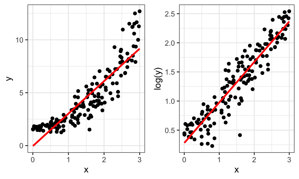
Figure 14.1: Impact of log-transforming \(y\).
Example 14.1 Consider the house price data introduced in Section 1.3.3. Figure 14.2 plots the median house sale price in each city against median income in each city. Although most of the points are in the lower left, there are some extreme values in the middle and upper right.
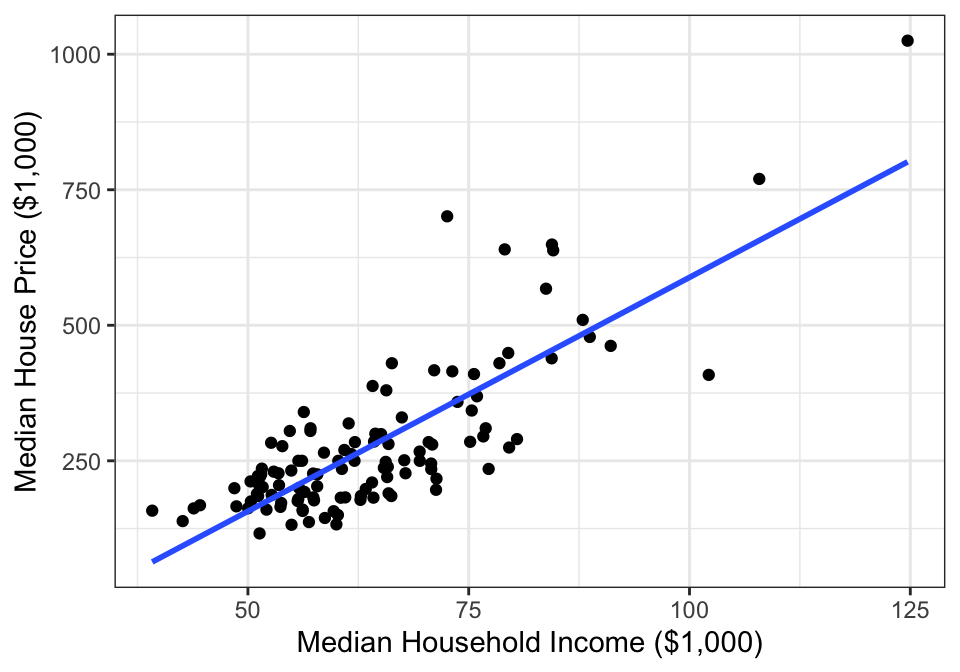
Figure 14.2: Median single-famly residence prices and median annual household income in U.S. metropolitan areas.
A residual plot (Figure 14.3) from this SLR model shows some evidence of non-linearity and non-constant variance present.
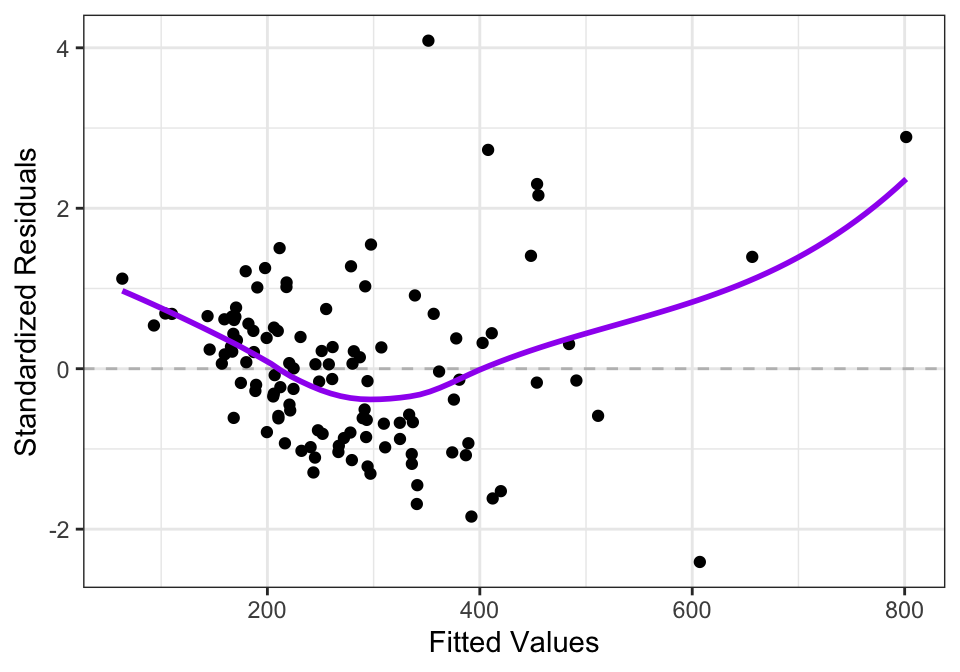
Figure 14.3: Residuals from SLR model of median single-famly residence prices as a function of median annual household income in U.S. metropolitan areas.
If we apply a log transform to median sale price, the data then look like Figure 14.4.
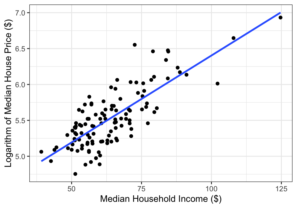
Figure 14.4: Logarithm of median single-famly residence prices and median annual household income in U.S. metropolitan areas.
The residual plot then looks like:
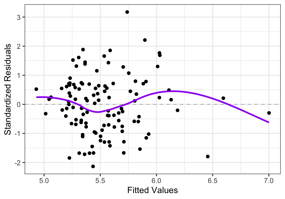
Figure 14.5: Residuals from SLR model of logarithm of median single-famly residence prices as a function of median annual household income in U.S. metropolitan areas.
Notice how in Figure 14.5, the values on the left hand side are more evenly spread out vertically than in Figure 14.3. The logarithm transform of the housing prices leads to less heteroscedasticity in the residuals. The trend line in Figure 14.3 also shows evidence of non-linearity, while the trend line in Figure 14.5 is closer to being flat, indicating less violation of the linearity assumption.
14.2.1 Interpreting a Model with \(\log Y\)
It’s important to remember that applying a transform on \(Y\) will change the interpretation of all of the model parameters. The \(\beta_j\) now represent differences in \(E[f(Y_i)]\), not in \(E[Y_i]\).
If the function \(f()\) is chosen to be the logarithm, then we can interpret \(\beta_j\) in terms of the geometric mean of \(Y\). Scientifically, using \(\log(Y_i)\) in place of \(Y_i\) is often appropriate for outcomes that operate on a multiplicative scale. Concentrations of pollution in the air or biomarkers in the blood are two examples of this.
The geometric mean is a measure of central tendency that is defined as: \[\begin{align*} GeoMean(x_1, \dots, x_n) &= \sqrt[n]{x_1 \times x_2 \times \dots \times x_n} \\ &= (x_1 \times x_2 \times \dots \times x_n)^{1/n} \end{align*}\]
The geometric mean is only define for positive numbers and is always smaller than the arithmetic mean (the usual “average”). It has the advantage of being more robust to outliers than the arithmetic mean and is also useful when there are multiplicative changes in a variable.
To connect the geometric mean to regression models with \(\log(Y)\) as the outcome, we first rewrite the geometric mean as: \[\begin{align*} GeoMean(x_1, \dots, x_n) &= \exp\left(\log\left[(x_1 \times x_2 \times \dots \times x_n)^{1/n}\right]\right)\\ &= \exp\left(\frac{1}{n} \left[\log(x_1) + \log(x_2) + \dots + \log(x_n)\right]\right) \end{align*}\] This relationship shows that \(\exp(\E[\log(X)])\) can be interpreted as the geometric mean of a random variable \(X\).
This means that in the model \[\log(Y) = \beta_0 + \beta_1x_{1} + \epsilon\] we have \[\beta_1 = \E[\log(Y) | x_1=x + 1] - \E[\log(Y) | x_1=x] \] Taking the exponential of both sides, we have \[\begin{align*} \exp(\beta_1) & = \exp\left(\E[\log(Y) | x_1=x + 1] - \E[\log(Y) | x_1=x]\right)\\ &=\frac{\exp(\E[\log(Y) | x_1=x + 1])}{\exp(\E[\log(Y) | x_1=x])}\\ &=\frac{GeoMean(Y | x_1 = x+ 1)}{GeoMean(Y | x_1 = x)} \end{align*}\] Thus, \(\exp(\beta_1)\) is the multiplicative difference in geometric mean of \(Y\) for a 1-unit difference in \(x_{1}\)
Example 14.2 In an SLR model with the logarithm of median house price as the outcome and median income (in thousands of dollars) as the predictor variable, the estimated value of \(\hat\beta_1\) is 0.024 (95% CI: 0.020, 0.028). Since \(exp(0.024) = 1.024\), this means that a difference of $1,000 in median income between cities is associated with a a 2.4% higher geometric mean sale price.
14.2.2 Other transformations
Other transformations are possible, such as square root (\(\sqrt{y}\)) and the inverse transform (\(1/y\)). In certain circumstances, these can solve issues of non-constant variances. However, they also make interpreting the regression coefficients more difficult than with the log transform.
14.3 Transformations on \(X\)
14.3.1 Transformations on \(X\)
In addition to transforming the outcome variable, we can transform the predictor variables. Common transformations for \(x\)’s are:
14.3.2 Log Transforming \(x\)’s
Replacing \(x_j\) with \(\log(x_j)\) can sometimes fix problems with non-linearity in the relationship. This is useful when additive differences in \(Y\) are associated with multiplicative differences in \(x_j\). It’s important to note that transforming predictor variables alone is usually not sufficient to fix non-constant variance; that typically requires a transformation on the outcome variable.
Example 14.3 Figure 14.6 shows the fuel efficiency of cars by engine size (data are from mpg.) We previously looked at this data as a candidate for an interaction model (Example 11.4), but the smooth in Figure 14.6 suggests that a transformation on engine size might also be appropriate.
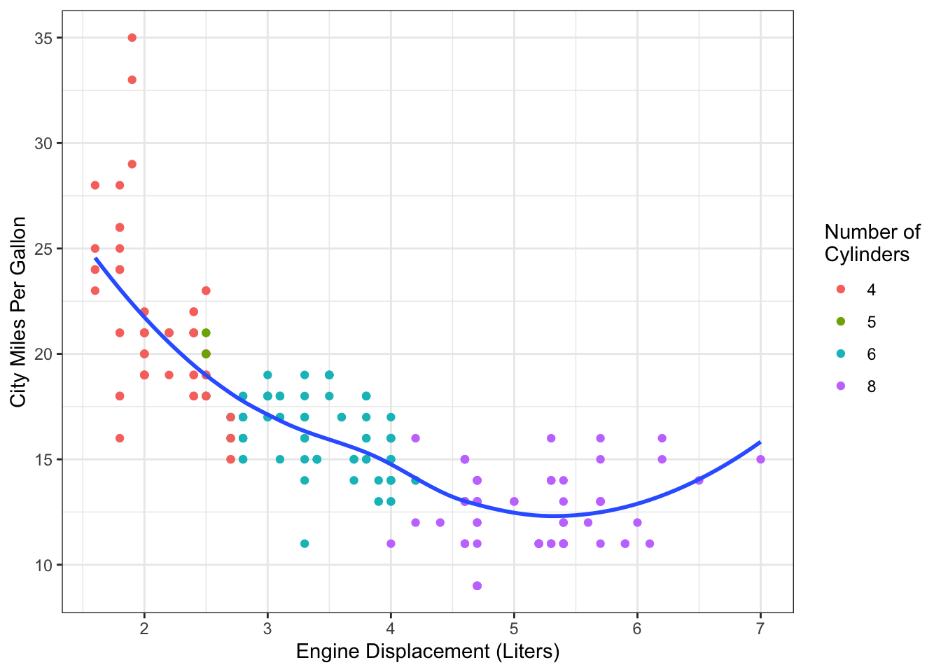
Figure 14.6: Fuel efficiency data from mpg dataset.
Figure 14.7 shows the same data, but with a log-transform of the predictor variable. The relationship now looks much more linear than it did before the transform.
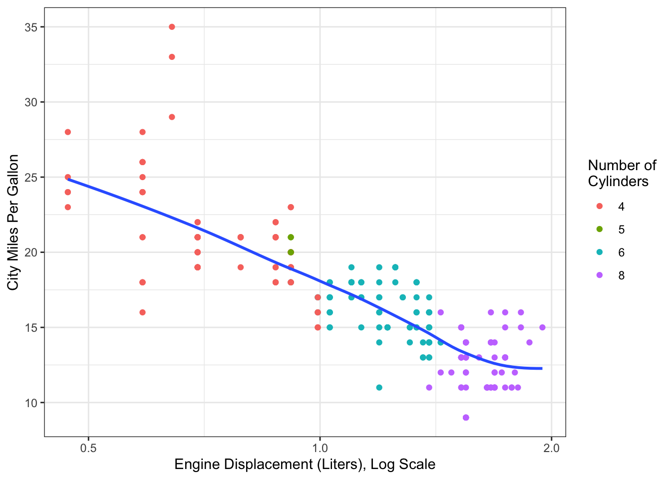
Figure 14.7: Fuel efficiency data from mpg dataset, with log transform for engine displacement.
If we log-transform the predictor variable, then we are essentially fitting the model: \[\begin{equation} Y_i = \beta_0 + \beta_1\log(x_{i1}) + \epsilon_i \tag{14.1} \end{equation}\] In (14.1), \(\beta_1\) is the difference in \(\E[Y_i]\) for a 1-unit difference in \(log(x_{i1})\). Since \(log(x) + 1 = log(x) + log(e) = log(x*e)\), a 1-unit difference in \(\log(x_{i1})\) is equivalent to an \(e\)-fold multiplicative difference in \(x_{i1}\). (An \(e\)-fold difference means multiplying the current value by \(e \approx 2.718\)).
Example 14.4 To fit an SLR model to the data in Figure 14.7, we could create a new variable is the log-transformed value of displ. Or, we can do the log transform within the call to lm():
mpg_logx_lm <- lm(hwy~log(displ), data=mpg)
tidy(mpg_logx_lm, conf.int=TRUE)
## # A tibble: 2 × 7
## term estimate std.error statistic p.value conf.low conf.high
## <chr> <dbl> <dbl> <dbl> <dbl> <dbl> <dbl>
## 1 (Intercept) 38.2 0.762 50.1 1.99e-126 36.7 39.7
## 2 log(displ) -12.6 0.618 -20.3 1.66e- 53 -13.8 -11.4In this model, the point estimates (and 95% CI) for \(\hat\beta_0\) and \(\hat\beta_1\) are 38.2 (36.7, 39.7) and -12.6 (-13.8, 11.4), respectively. From this, we can conclude that an \(e\)-fold difference in engine size is associated with 12.6 (11.4, 13.8) lower miles per gallon on the highway.
14.4 Log-transforming \(x\) and \(Y\)
In addition to transforming only \(x\) or only \(Y\), we can fit a model with a transform applied to both. This is most commonly done using a logarithm transform on both \(x\) and \(Y\). The SLR model becomes
\[\begin{equation} \E[\log(Y_i)]= \beta_0 + \beta_1\log(x_i). \tag{14.2} \end{equation}\]
By exponentiating both sides of (14.2), we obtain \[\begin{align} e^{\E[\log(Y_i)]} &= e^{\beta_0}e^{\beta_1\log(x_i)} =e^{\beta_0}x_i^{\beta_1} \tag{14.3} \end{align}\] Equation (14.3) shows that \(\exp(\beta_1)\) is the multiplicative difference in the geometric mean of \(Y\) for an \(e\)-fold difference in \(x\). Conceptually, this means that multiplicative differences in \(x\) are related to multiplicative differences in (the geometric mean of) \(Y\). Thus, the log-log model (14.2) can work particularly well for an exponential or growth model.
Example 14.5 Figure 14.8 shows the stock price and market capitalization for companies on the S&P 500. The data are concentrated in the bottom left, with only a few companies with large market capitalizations or high stock prices. Based on this scatterplot, a linear regression model that uses these values (market capitalization and stock price) directly would not fit the data well.
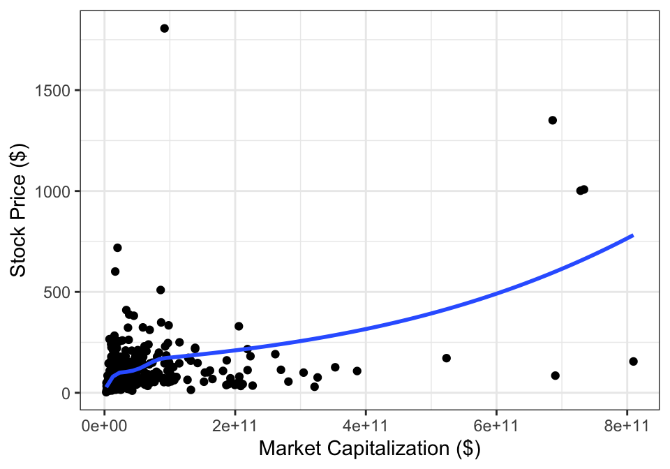
Figure 14.8: Stock prices and market capitalization.
But if we log-transform both variables, than we get Figure 14.9. After the transformation, the relationship between the variables looks to be much more linear.
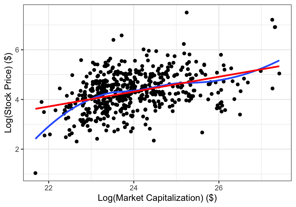
Figure 14.9: Stock prices and market capitalization, after log-transforming both variables. The red line is shows the SLR line and the blue curve is a smooth through the data.
We can estimate the model coefficients by fitting the model:
sp_lm1 <- lm(log(price)~log(market_cap), data=sp500)tidy(sp_lm1, conf.int=TRUE) %>%
select(-c(p.value, statistic)) %>%
rename_with(tools::toTitleCase) %>%
kable(digits=3)| Term | Estimate | Std.error | Conf.low | Conf.high |
|---|---|---|---|---|
| (Intercept) | -2.866 | 0.761 | -4.362 | -1.370 |
| log(market_cap) | 0.299 | 0.032 | 0.237 | 0.362 |
The estimated line is \(\widehat{\log y_i} = -2.87 + 0.30\log x_i\), which leads to a non-linear relationship on the original scale:

14.5 Polynomial Models
14.5.1 Polynomial Regression
While the log transform can be useful, it isn’t always appropriate for a set of data. Sometimes the relationship between \(\E[Y]\) and \(x\) is best modeled using a polynomial.
Example 14.6 Consider again the fuel efficiency data in Figure 14.6. Instead of log-transforming \(x\), we could instead use a quadratic polynomial to reprsent the relatioship between fuel efficiency and engine size. This leads to the curve shown in Figure 14.10
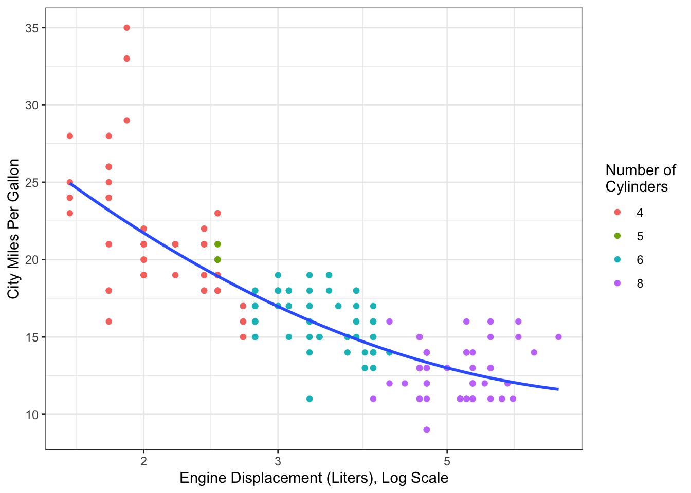
Figure 14.10: Fuel efficiency data from mpg dataset. Curve estimated using a quadratic polynomial for engine displacement.
When using a polynomial transformation, we are still fitting a linear regression model–recall that the term “linear” refers to the coefficients, not the predictors. A quadratic polynomial model can be written: \[\begin{equation} Y_i = \beta_0 + \beta_1 x_i + \beta_2 x_i^2 + \epsilon_i. \tag{14.4} \end{equation}\] Model (14.4) looks like our standard multiple linear regression model, we just now have \(x^2\) as one of the predictor variables.
Since \(x_i\) shows up twice in model (14.4), parameter interpretation are more complicated than in regular MLR models. \(\beta_1\), the coefficient for \(x_i\), can no longer be interpreted as the difference in average value of \(Y\) for a one-unit difference in \(x_i\) (adjusting for all other predictors). This is because a 1-unit change in \(x_i\) also means that there must be a difference in the \(x_i^2\) term. Because of this, in polynomial models it is common to not interpret the individual parameters. Instead, focus is on the overall model fit and estimated mean (or equivalently, predicted values).
14.5.2 Estimating Polynomial Models
To estimate coefficients for a polynomial model, quadratic (and higher-order) terms can be added directly to the model, like in (14.4). This can be accomplished in R by adding the terms I(x^2) to the model formula. (The I() is necessary to indicate that you are performing a transformation of the variable x).
Example 14.7 We can fit a quadratic model to the data from Example 14.6 by running the code:
mpg_quad <- lm(hwy~displ + I(displ^2), data=mpg)
summary(mpg_quad)
##
## Call:
## lm(formula = hwy ~ displ + I(displ^2), data = mpg)
##
## Residuals:
## Min 1Q Median 3Q Max
## -6.6258 -2.1700 -0.7099 2.1768 13.1449
##
## Coefficients:
## Estimate Std. Error t value Pr(>|t|)
## (Intercept) 49.2450 1.8576 26.510 < 2e-16 ***
## displ -11.7602 1.0729 -10.961 < 2e-16 ***
## I(displ^2) 1.0954 0.1409 7.773 2.51e-13 ***
## ---
## Signif. codes: 0 '***' 0.001 '**' 0.01 '*' 0.05 '.' 0.1 ' ' 1
##
## Residual standard error: 3.423 on 231 degrees of freedom
## Multiple R-squared: 0.6725, Adjusted R-squared: 0.6696
## F-statistic: 237.1 on 2 and 231 DF, p-value: < 2.2e-16This yields estimated coefficients like usual, from which we can calculate the estimated model, make predictions, and more.
In practice, using polynomial terms directly in the model can lead to some stability issues due to correlation between the predictors. (The values of \(x\) are naturally highly correlated with the values of \(x^2\), \(x^3\), etc.) Instead, it’s better to use orthogonal polynomials. The mathematical details of creating orthogonal polynomials is outside the scope of this book, but they are easy to implement in R. Instead of including x + I(x^2) + I(x^3) in the model formula, simply use poly(x, 3). The poly() function creates the orthogonal polynomials for you, providing better stability in coefficient estimates and reducing the likelihood of typographical mistakes.
Example 14.8 In our fuel efficiency data example, we can fit an equivalent model using the code:
mpg_quad_v2 <- lm(hwy~poly(displ, 2), data=mpg)
summary(mpg_quad_v2)
##
## Call:
## lm(formula = hwy ~ poly(displ, 2), data = mpg)
##
## Residuals:
## Min 1Q Median 3Q Max
## -6.6258 -2.1700 -0.7099 2.1768 13.1449
##
## Coefficients:
## Estimate Std. Error t value Pr(>|t|)
## (Intercept) 23.4402 0.2237 104.763 < 2e-16 ***
## poly(displ, 2)1 -69.6264 3.4226 -20.343 < 2e-16 ***
## poly(displ, 2)2 26.6042 3.4226 7.773 2.51e-13 ***
## ---
## Signif. codes: 0 '***' 0.001 '**' 0.01 '*' 0.05 '.' 0.1 ' ' 1
##
## Residual standard error: 3.423 on 231 degrees of freedom
## Multiple R-squared: 0.6725, Adjusted R-squared: 0.6696
## F-statistic: 237.1 on 2 and 231 DF, p-value: < 2.2e-16If we compare the output from the two models, we can see that the coefficient estimates differ. This is because the quadratic polynomial is being represented in two different (but mathematically equivalent) ways. The overall model fit is the same for both models, which we can see in the identical values for \(\hat\sigma\), \(R^2\), and Global \(F\) statistic. The fit from both model is plotted in Figure 14.10.
14.5.3 Testing in Polynomial Models
Like with interaction models, hypothesis testing in polynomial models requires some care when setting up appropriate null hypotheses. When considering which parameters to test, we want to keep an important rule in mind: lower-order terms must always remain in the model.
This means, if we have a quadratic model like (14.4), then we could test \(H_0: \beta_2 = 0\), but we would not want to test \(H_0: \beta_1 =0\). Removing the lower order terms (e.g. \(x\)) but leaving higher-order terms (e.g., \(x^2\)) puts strong mathematical constraints on what remains, in a manner similar to fitting an SLR model but forcing the intercept to be zero.
This means the following hypothesis tests are valid for an MLR model with polynomial terms:
- Testing only the highest order \(x\) terms
- Testing all of the \(x\) terms
- Testing some of the \(x\) terms, starting with the highest order term and including the next lower-order terms from there.
In the case of the model \[\begin{equation} Y_i = \beta_0 + \beta_1 x_i + \beta_2 x_i^2 + \beta_3x_i^2 + \epsilon_i. \tag{14.4} \end{equation}\] this means the following tests are appropriate:
- \(H_0: \beta_3 = 0\)
- \(H_0: \beta_1 = \beta_2 = \beta_3 = 0\)
- \(H_0: \beta_2 = \beta_3 = 0\)
Like with other MLR models, these hypotheses can be tested using a T test, Global F-test, and Partial F-test, respectively.
Example 14.9 Suppose we fit a cubic model to the fuel efficiency data. We can test whether the cubic model is a better fit compared to the quadratic model using the null hypothesis \(H_0: \beta_3 = 0\). There are two equivalent ways to test this: (i) looking at the \(t\)-test corresponding to \(\beta_3\) directly and (ii) using an F-test to compare the cubic model to the quadratic model.
mpg_cubic <- lm(hwy~poly(displ, 3), data=mpg)
tidy(mpg_cubic)
## # A tibble: 4 × 5
## term estimate std.error statistic p.value
## <chr> <dbl> <dbl> <dbl> <dbl>
## 1 (Intercept) 23.4 0.222 105. 1.11e-196
## 2 poly(displ, 3)1 -69.6 3.40 -20.5 1.03e- 53
## 3 poly(displ, 3)2 26.6 3.40 7.82 1.89e- 13
## 4 poly(displ, 3)3 6.65 3.40 1.95 5.18e- 2From the tidy() output, we have do not have evidence to reject the null hypothesis that \(\beta_3 = 0\) (\(p=0.052\)). We would obtain the same result using an F-test:
anova(mpg_quad_v2, mpg_cubic)## Analysis of Variance Table
##
## Model 1: hwy ~ poly(displ, 2)
## Model 2: hwy ~ poly(displ, 3)
## Res.Df RSS Df Sum of Sq F Pr(>F)
## 1 231 2706.1
## 2 230 2661.8 1 44.229 3.8217 0.0518 .
## ---
## Signif. codes: 0 '***' 0.001 '**' 0.01 '*' 0.05 '.' 0.1 ' ' 114.5.4 Predicting Polynomial Models
When making predictions from polynomial models, we can use predict() like with regular MLR models. Since we define the polynomial transformation within the model fit (i.e. by including poly(x, 3) instead of creating new columns in the data frame), we only need to provide the predictor variable column in the prediction data frame.
Example 14.10 Let’s use our quadratic model for the fuel efficiency data to predict the average highway fuel efficiency for a vehicle with a 6 L engine. We can do this by calling predict():
predict(mpg_quad_v2,
        newdata=data.frame(displ=6),
        interval="prediction")
## fit lwr upr
## 1 18.11906 11.245 24.99313Our model estimates that a vehicle with a 6-L engine will get 18.1 mpg (95% PI: 11.2, 25.0) on the highway.
14.6 Splines
Polynomial models provide flexibility over models that only include linear terms for the predictors. While it’s theoretically possible to model any function as a polynomial if you include enough terms (think of a Taylor series expansion), going beyond quadratic terms in a regression often runs into stability problems. In the highest and lowest ranges of the data (the “tails” of the data), the values can be highly variable, leading to poor fit in those areas.
Instead, we can use a flexible form for \(x\) that doesn’t have such erratic tail behavior. Splines provide one such approach. Essentially, we can think of splines as simple building blocks that we can use to form more complicated functions. Figure 14.11 shows four standard splines14 that can be used to represent different functions of \(x\). The number of splines is typically called the degrees of freedom for the spline15.
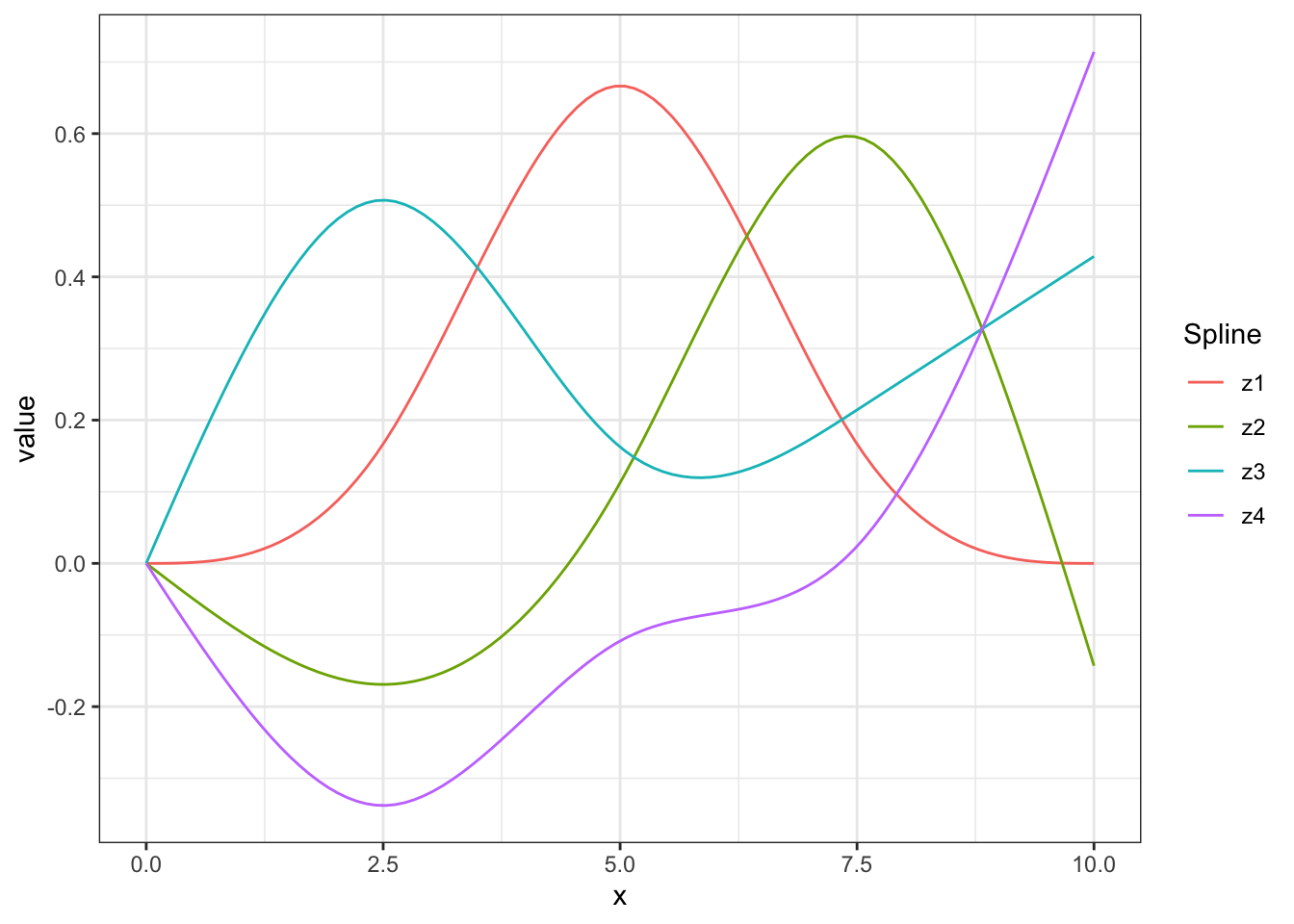
Figure 14.11: Natural cubic splines with \(df=4\).
If we have \(df=4\) splines \(z_1\), \(z_2\), \(z_3\), and \(z_4\), like in Figure 14.11 , we can fit the model: \[Y_i = \beta_0 + \beta_1z_1 + \beta_2z_2 + \beta_3z_3 + \beta_4z_4 + \epsilon_i\]
Figure 14.12 shows one possible combination of these splines to create a single curve. In this case, the curve is \(1s_1 -0.5s_2 + 0.2s_3 + 0.4s_4\), where \(s_j\) are the different splines from Figure 14.11. The more splines, the more flexible the curve that can be fit.
It’s important to remember that like with polynomial models, we cannot interpret \(\beta_1\) alone. A change in the value of \(x\) would change all of the values \(z_1\), \(z_2\), \(z_3\), \(z_4\). Thus, splines are best used when coefficient interpretation is not needed–such as when prediction is the goal, or when using a variable for adjustment and inferential interest is on another variables.
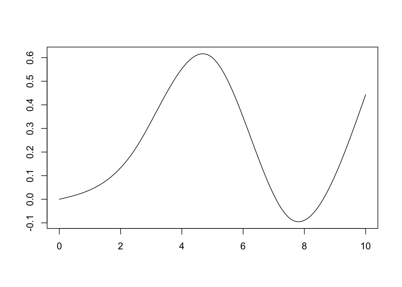
Figure 14.12: Example linear combination of splines to form a cuve.
The more splines, the more flexible the curve that can be fit.
- Cannot interpret \(\beta_1\) alone, since \(z_1\), \(z_2\), \(z_3\), \(z_4\) all change together depending on value of \(x\)
- Splines are best used when coefficient interpretation is not needed. Such as:
- Spline variable is just for adjustment, and predictor of interest is a different variable
- Prediction of \(y\) is goal
Example 14.11 Consider the baseball hit data from Example 1.7 and plotted again in Figure 14.13. These data show a non-linear trend that doesn’t easily match to a logarithmic or polynomial function. Instead, we can include a spline fit, like the one shown in Figure 14.13.
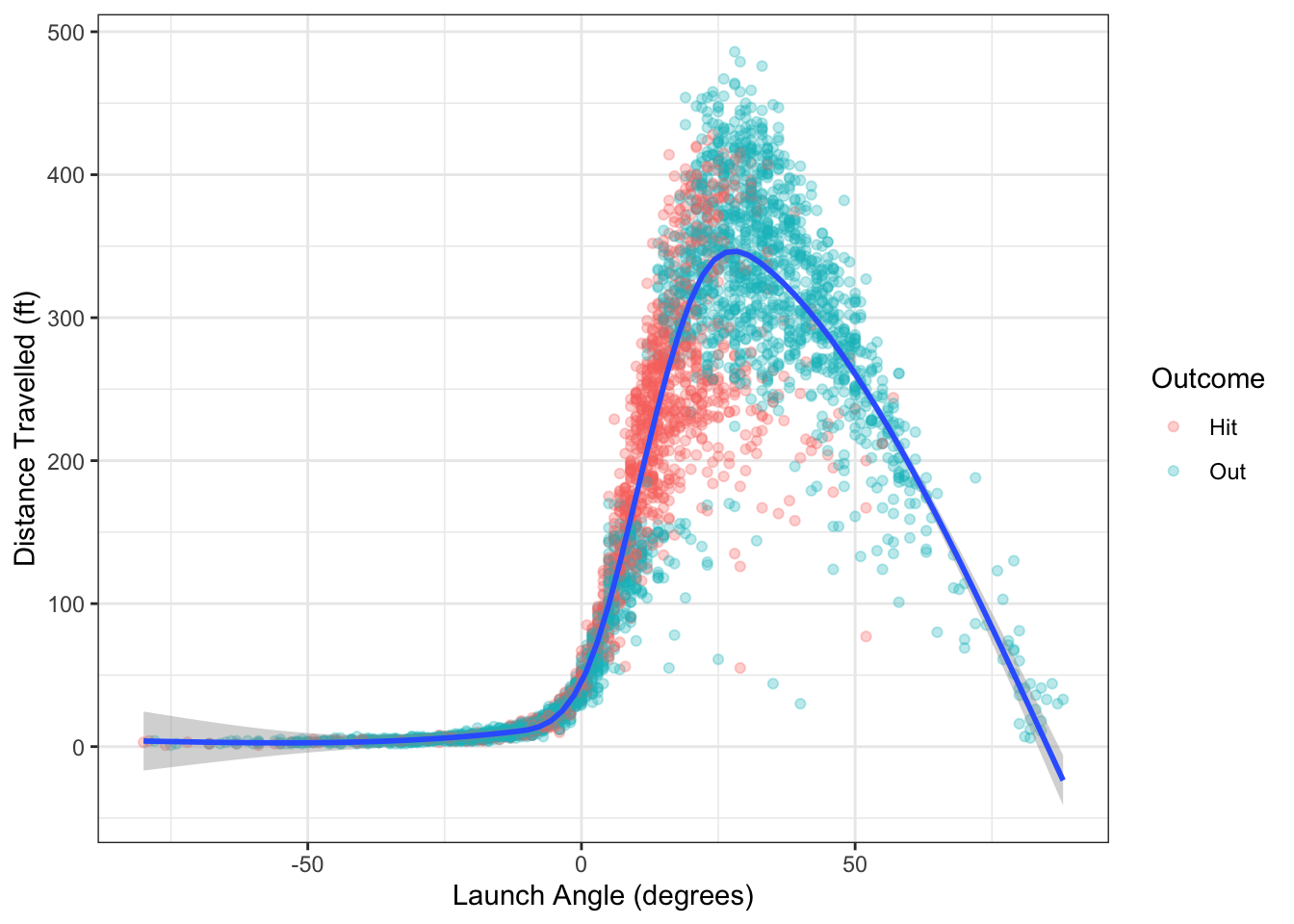
Figure 14.13: Distance travelled and launch angle for balls in play from Colorado Rockies in 2019.
To fit this model, we run the code:
bb_lm_spline <- lm(hit_distance~ns(launch_angle, 6), data=bb)
summary(bb_lm_spline)
##
## Call:
## lm(formula = hit_distance ~ ns(launch_angle, 6), data = bb)
##
## Residuals:
## Min 1Q Median 3Q Max
## -290.990 -11.524 0.195 17.584 151.414
##
## Coefficients:
## Estimate Std. Error t value Pr(>|t|)
## (Intercept) 3.894 10.528 0.370 0.71152
## ns(launch_angle, 6)1 13.086 9.911 1.320 0.18679
## ns(launch_angle, 6)2 208.536 11.369 18.343 < 2e-16 ***
## ns(launch_angle, 6)3 358.980 10.694 33.567 < 2e-16 ***
## ns(launch_angle, 6)4 306.762 7.059 43.456 < 2e-16 ***
## ns(launch_angle, 6)5 118.920 23.562 5.047 4.7e-07 ***
## ns(launch_angle, 6)6 -25.680 9.890 -2.597 0.00945 **
## ---
## Signif. codes: 0 '***' 0.001 '**' 0.01 '*' 0.05 '.' 0.1 ' ' 1
##
## Residual standard error: 44.11 on 3808 degrees of freedom
## (31 observations deleted due to missingness)
## Multiple R-squared: 0.9026, Adjusted R-squared: 0.9025
## F-statistic: 5883 on 6 and 3808 DF, p-value: < 2.2e-1614.7 Exercises
Exercise 14.1 Compare the cubic model from Example 14.9 to a model that includes engine displacement as only a linear term. State the null and alternative hypotheses, the test statistic, \(p\)-value, and a conclusion statement.