Chapter 11 Indicators and Interactions
\(\newcommand{\E}{\mathrm{E}}\) \(\newcommand{\Var}{\mathrm{Var}}\) \(\newcommand{\bmx}{\mathbf{x}}\) \(\newcommand{\bmH}{\mathbf{H}}\) \(\newcommand{\bmI}{\mathbf{I}}\) \(\newcommand{\bmX}{\mathbf{X}}\) \(\newcommand{\bmy}{\mathbf{y}}\) \(\newcommand{\bmY}{\mathbf{Y}}\) \(\newcommand{\bmbeta}{\bm{\beta}}\) \(\newcommand{\XtX}{\bmX^\mT\bmX}\) \(\newcommand{\mT}{\mathsf{T}}\) \(\newcommand{\XtXinv}{(\bmX^\mT\bmX)^{-1}}\)
11.1 Categorical Variables
So far, we have focused on predictor variables that were either continuous variables or binary variables. There is one other important variable type that can be used as a predictor variable: categorical variables.
Categorical variables are variables that can take discrete, unordered, values. Examples include plant species, blood type, or position on a sports team. Binary variables are a special case of categorical variables that have only two possible values.
11.2 Indicator Variables
Categorical variables aren’t inherently numeric, and so we must come up with a way to code them numerically to include in a regression model. The standard method for doing this is to create a series of \(K-1\) binary indicator variables to represent \(K\) different categories.
Suppose we have a variable, \(z_i\), that takes three values: \(A\), \(B\), or \(C\). We can define two binary indicators \(x_{iB}\), and \(x_{iC}\) that take values:
\[\begin{align*} x_B = \begin{cases} 1 & \text{ if observation $i$ is in category $B$}\\ 0 & \text{ if observation $i$ is not in category $B$}\end{cases} \end{align*}\]
\[\begin{align*} x_C = \begin{cases} 1 & \text{ if observation $i$ is in category $C$}\\ 0 & \text{ if observation $i$ is not in category $C$}\end{cases} \end{align*}\]
Together these two variables can represent three categories. The different combinations are summarized in Table 11.1. Observations that have \(z_i = A\) have \((x_{iB}, x_{iC}) = (0, 0)\). Observations that have \(z_i = B\) have \((x_{iB}, x_{iC}) = (1, 0)\). Observations that have \(z_i = C\) have \((x_{iB}, x_{iC}) = (0, 1)\).
| \(z\) | \(x_B\) | \(x_C\) |
|---|---|---|
| A | 0 | 0 |
| B | 1 | 0 |
| C | 0 | 1 |
In this setup, the category A is known as the reference category. The other groups (B and C) are coded as differences from the A group, which corresponds to a value of 0 for all of the indicators. The overall model fit does not depend on which category is chosen as reference. However, interpretations of the indicator coefficients change depending on which variable is chosen as the reference category.
Suppose we create an MLR model with three predictor variables: a continuous variable \(x_{i1}\) and the two indicator variables \(x_{iB}\) and \(x_{iC}\). The equation for the full model:
\[\begin{equation} Y_i = \beta_0 + \beta_1x_{i1} + \beta_2x_{iB} + \beta_3x_{iC} + \epsilon_i \tag{11.1} \end{equation}\]
Using (11.1), we can write three different models for \(Y_i\), one for each value of \(z_i\):
- Observations with \(z_i = A\) have the equation \[Y_i = \beta_0 + \beta_1x_{i1} + \epsilon_i\]
- Observations with \(z_i = B\) have the equation \[Y_i = \beta_0 + \beta_1x_{i1} + \beta_2 + \epsilon_i\]
- Observations with \(z_i = A\) have the equation \[Y_i = \beta_0 + \beta_1x_{i1} + \beta_3 + \epsilon_i\]
The indicators allow for different intercepts for each model. Observations with \(z = A\) have intercept \(\beta_0\). Observations with \(z = B\) have intercept \(\beta_0 + \beta_2\). Observations with \(z = C\) have intercept \(\beta_0 + \beta_3\). This means that we can interpret the coefficient for an indicator for category “k” as the difference in the average value of the outcome, comparing observations in category “k” to observations in the reference category that have the same values for the other variables in the model.
Indicator variables can be used for an arbitrary number of categories. There is always one less indicator variable than number of categories. For a categorical variable with \(K\) different categories: \[\begin{align*} x_1 &= \begin{cases} 1 & \text{ if category 2} \\ 0 & \text{if not category 2} \end{cases}\\ x_2 &= \begin{cases} 1 & \text{ if category 3} \\ 0 & \text{if not category 3} \end{cases}\\ &\vdots\\ x_{K-1} &= \begin{cases} 1 & \text{ if category K} \\ 0 & \text{if not category K} \end{cases} \end{align*}\]
There is an important restriction on the indicator variable values: only one of them can be non-zero at a time. This preserves the interpretation of each coefficient as the difference in the average value of the outcome, comparing the indicator category to the reference category.
The approach described here for indicator variables is sometimes called “dummy coding” of a categorical variable, since there is a separate indicator for each comparison. An alternative, which we will not discuss further here, is “effect coding”.
Example 11.1 Using the photosynthesis data introduced in Section 10, we can fit a model that adjusts for soil water content and tree species. For the time being, let’s restrict to three species: balsam fir (coded as "abiba"), Jack Pine (codede as "pinba"), and Red Oak (coded as "queru").
We can plot the data separately by species:

Or in a single plot, but color points by species:

We can write the MLR model for this data as \[\begin{equation} Y_i = \beta_0 + \beta_1x_{i1} + \beta_2x_{i2} + \beta_3x_{i3} + \epsilon_i \tag{11.2} \end{equation}\] where the variables are: \[\begin{align*} x_1 &= \begin{cases} 1 & \text{ if `species` is `pinba`} \\ 0 & \text{ if `species` is not `pinba`}\end{cases}\\ x_2 &= \begin{cases} 1 & \text{ if `species` is `queru`} \\ 0 & \text{ if `species` is not `queru`}\end{cases}\\ x_3 &= \text{Soil Water Content} \end{align*}\] We can interpret the model parameters as:
- \(\beta_0\) – The average photosynthesis output for Balsam Fir trees with a soil water content ratio of zero.
- \(\beta_1\) – The difference in average photosynthesis output comparing Jack Pine trees to Balsam Fir trees with the same soil water content ratio.
- \(\beta_2\) – The difference in average photosynthesis output comparing Red Oak trees to Balsam Fir trees with the same soil water content ratio.
- \(\beta_3\) – The difference in average photosynthesis output for a 1-unit difference in soil water content ratio, among trees of the same species.
11.3 Indicators in R
For a categorical variable (class is character or factor), R will automatically create the indicator variables. The category that comes first alphabetically is chosen as the reference category (unless a different reference is explicitly set for a factor variable.) The variables are given a name that is a combination of the variable name and the category label.
The following code output shows the model matrix (\(\bmX\)) that R creates for a model that adjusts for soil water content and species.
X <- model.matrix(~species + soil_water, data=photo_small)
head(X)
## (Intercept) speciespinba speciesqueru soil_water
## 1 1 0 0 0.1813521
## 2 1 0 0 0.1825371
## 3 1 1 0 0.1766267
## 4 1 1 0 0.1180401
## 5 1 1 0 0.1589861
## 6 1 0 1 0.203437211.4 Testing Categorical Variables
To test whether there is a relationship between the average value of the outcome variable and a categorical variable, we should conduct a Partial F-Test that compares a reduced model without any of the indicator variables to a full model that contains all of them.
Since the indicator variables each individually only compare a single category level to the reference, testing one individually does not account for the role of the other indicator variables in the model. We want to test all of them at once, not a variable one-by-one.
Example 11.2 We can fit the model described in Example 11.1. Is there evidence of a difference in photosynthesis output by species?
We first fit the model (11.2) by running the code:
photo_lm <- lm(photosyn~species + soil_water, data=photo_small)We can view each of the coefficient estimates using tidy():
tidy(photo_lm, conf.int=T)## # A tibble: 4 × 7
## term estimate std.error statistic p.value conf.low conf.high
## <chr> <dbl> <dbl> <dbl> <dbl> <dbl> <dbl>
## 1 (Intercept) 1.09 0.937 1.17 2.44e- 1 -0.750 2.94
## 2 speciespinba 7.00 0.810 8.64 3.94e-16 5.41 8.60
## 3 speciesqueru 4.54 0.749 6.07 4.09e- 9 3.07 6.02
## 4 soil_water 32.4 4.59 7.05 1.35e-11 23.3 41.4Our question of interest corresponds to the null and alternative hypothesis:
- \(H_0\): There is no relationship between average photosynthesis output and species, among trees with the same soil water content ratio.
- \(H_A\): There is a relationship between average photosynthesis output and species, among trees with the same soil water content ratio.
We fit the reduced model and compare to the full model:
photo_lm_reduced <- lm(photosyn~soil_water, data=photo_small)
anova(photo_lm_reduced, photo_lm)
## Analysis of Variance Table
##
## Model 1: photosyn ~ soil_water
## Model 2: photosyn ~ species + soil_water
## Res.Df RSS Df Sum of Sq F Pr(>F)
## 1 290 7754.2
## 2 288 6157.7 2 1596.5 37.335 3.826e-15 ***
## ---
## Signif. codes: 0 '***' 0.001 '**' 0.01 '*' 0.05 '.' 0.1 ' ' 1We reject the null hypothesis that there is no relationship between average photosynthesis output and species, among trees with the same soil water content ratio (\(f=37.3, p<0.0001\)).
11.5 Interactions in Regression
Indicator variables allow for the intercept in the model to vary by different categories. But what if we want to allow the slopes to vary among different groups? To do this, we can include an interaction term in the model.
Example 11.3 One factor that affects fuel economy in passenger vehicles is the size of the engine. Figure 11.1 shows the highway miles per gallon for vehicles, as a function of their engine size.
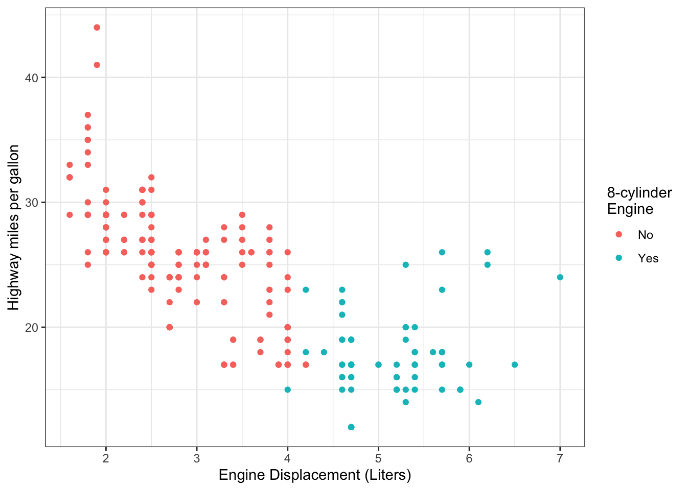
Figure 11.1: Fuel efficiency and engine size in a sample of vehicles.
In Figure 11.1, it seems evident that the relationship between fuel efficiency and engine size differs between engines with 8 cylinders and those with fewer cylinders. To do this, we can construct an MLR model with an interaction between engine size and an indicator of having 8 cylinders.
Define the variables to be:
- \(Y_i =\) Highway MPG
- \(x_{i1} =\) Engine Displacement
- \(x_{i2} =\) Indicator of 8-cylinder engine (0=no, 1=yes)
The model we can fit is: \[\begin{equation} Y_i = \beta_0 + \beta_1x_{i1} + \beta_2x_{i2} + \beta_3x_{i1}x_{i2} + \epsilon_i \tag{11.3} \end{equation}\] For vehicles with <8 cylinders (\(x_{i2}=0\)), the model becomes: \[\E[Y_i] = \beta_0 + \beta_1x_{i1}\] For vehicles with 8 cylinders (\(x_{i2}=1\)), the model becomes: \[\E[Y_i] = (\beta_0 + \beta_2) + (\beta_1 + \beta_3)x_{i1} \] The parameter \(\beta_3\) allows the slope to differ between the two groups defined by \(x_{i2}\).
Graphically, we can represent this by having separate regression lines in the scatterplot:
## `geom_smooth()` using formula = 'y ~ x'
11.6 Interpreting Parameters in Interactions
For model with continuous \(x_1\) and binary \(x_2\), and an interaction between these terms, the MLR model is given above in (11.3). It’s important that any time an interaction term is added to a model, both variables are also included by themselves. This is called including the “main effects” for any variables that have “interaction effects”.
In the model (11.3), the “slope” for \(x_1\) depends on the value of \(x_2\)
- \(\beta_1\) is the difference in the average value of \(Y\) for a 1-unit difference in \(x_1\), among observations with \(x_2 = 0\).
- \(\beta_1 + \beta_3\) is the difference in the average value of \(Y\) for a 1-unit difference in \(x_1\), among observations with \(x_2 = 1\).
- \(\beta_3\) is the difference between observations with \(x_2= 1\) and \(x_2 = 0\) in the difference in the average value of \(Y\) for a 1-unit difference in \(x_1\).
The “intercept” for the model also depends on the value of \(x_2\)
- \(\beta_0\) is the average value of \(Y\) for observations with \(x_1 = 0\) and \(x_2=0\)
- \(\beta_0 + \beta_2\) is the average value of \(Y\) for observations with \(x_1=0\) and \(x_2=1\)
- \(\beta_2\) is the difference of the average value of \(Y\) when \(x_1=0\) between observations with \(x_2=1\) and \(x_2=0\)
11.7 Interactions in R
In R, interactions can be created using * in the formula. For example:
mpg_lm_interact <- lm(hwy~displ*cyl8, data=mpg)This code fits a model with the following variables:
displcyl8yes- Has value 1 if
cyl8is"yes" - Has value 0 if
cyl8is"no"
- Has value 1 if
displ:cyl8yes- Has the value of
displifcyl8is"yes" - Has the value of 0 if
cyl8is"no"
- Has the value of
It is possible to use the R formula displ + cyl8 + displ:cyl8, but using displ*cyl8 is shorter and almost always better.
Example 11.4 Is there a difference in the relationship between average highway MPG and engine size, comparing vehicles witht 8-cylinder engines compared to those without?
This corresponds to testing \(H_0: \beta_3 = 0\) versus \(H_A: \beta_3 \ne 0\) in Model (11.3). From the following model output,
tidy(mpg_lm_interact)## # A tibble: 4 × 5
## term estimate std.error statistic p.value
## <chr> <dbl> <dbl> <dbl> <dbl>
## 1 (Intercept) 39.5 1.03 38.3 1.08e-101
## 2 displ -4.92 0.361 -13.6 2.14e- 31
## 3 cyl8yes -28.5 3.75 -7.61 6.88e- 13
## 4 displ:cyl8yes 6.22 0.786 7.92 1.04e- 13we can see that the corresponding \(t\) statistic is 7.9 and the \(p\)-value is less than 0.0001. Thus, we would reject \(H_0\).
11.8 Interactions with 2 Continuous Variables
In addition to interactions between a continuous variable and a binary variable, interactions between two continuous variables can also be created.
For example, in the photosynthesis data, we could fit the model \[Y_i = \beta_0 + \beta_1x_{i1} + \beta_2x_{i2} + \beta_3x_{i1}x_{i2} + \epsilon_i\]
where:
- \(Y =\) photosynthesis output
- \(x_1 =\) soil water content
- \(x_2 =\) leaf temperature
For model with continuous \(x_1\) and continuous \(x_2\), the “slope” for \(x_1\) depends on the value of \(x_2\). \(\beta_1 + \beta_3x_2\) is the difference in the average value of \(Y\) for a 1-unit difference in \(x_1\). Analogously, the “slope” for \(x_2\) depends on the value of \(x_1\). \(\beta_2 + \beta_3x_1\) is the difference in the average value of \(Y\) for a 1-unit difference in \(x_2\)
11.9 More Complicated Interactions
More complicated forms for interactions are possible. Interactions can include categorical variables with more than 2 levels (e.g. species in the photosynthesis data). Interactions can also be created between three (or more) different variables, although it can be cumbersome to interpret the results.