Chapter 8 The Multiple Linear Regression (MLR) Model
\(\newcommand{\E}{\mathrm{E}}\) \(\newcommand{\Var}{\mathrm{Var}}\)
8.1 Multiple Linear Regression
Simple linear regression (SLR) gave us a tool to model the relationship between a single predictor variable (\(x_i\)) and an outcome (\(Y_i\)):
\[Y_i = \beta_0 + \beta_1x_{i} + \epsilon_i\] This has a clear drawback: most real-world outcomes are impacted by more than one variable. Multiple linear regression (MLR) extends SLR to include multiple predictor variables. Suppose we have a set of \(k\) predictor variables, whose values for the \(i\)th observation are denoted \(x_{i1}, \dots, x_{ik}\). The MLR model for an outcome \(Y_i\) as a function of these variables is:
\[\begin{equation} Y_i = \beta_0 + \beta_1x_{i1} + \beta_2x_{i2} + \dots + \beta_kx_{ik} + \epsilon_i \tag{8.1} \end{equation}\]
This chapter will explore how adding the additional predictor variables affects the interpretation of the coefficient parameters \(\beta_j\). In Chapter 9.2, we will see an alternative form of the MLR model that uses matrix algebra to simplify computations and directly use these properties to show properties of the parameter estimates.
The multiple linear regression model (8.1) has analogous assumptions to simple linear regression:
- \(E[\epsilon_i] = 0\)
- \(Var(\epsilon_i) = \sigma^2\)
- \(\epsilon_i\) are uncorrelated
As we will see, these assumptions means that the mathematical details of SLR extend readily to having more than one predictor variable. Section 12 discusses how to assess whether these assumptions are met for a given dataset, and what problems can occur when they are not.
For now, we will consider continuous and binary predictor variables. Section 11 explores categorical predictors and other transformations of continuous predictors are covered in Section 14. Section 8.2 presents an example model with one continuous predictor and one binary predictor; Section 8.3 presents an example model with two continuous predictors; and Section 8.4 discusses how to interpret parameters in a general moodel with an arbitrary number of predictor variables.
8.2 MLR Model 1: One continuous and one binary predictor
We first discuss an MLR model with one continuous predictor and one binary predictor. This setting has the advantage of being easy to represent graphically in a scatterplot.
Consider again the penguin data from Examples 2.7 and 2.8. We let body mass be the outcome, but now include both sex and flipper length as predictor variables. From the data plotted in Figure 8.1, we can see two trends:
- Penguins with longer flippers tend to have greater body mass
- Male penguins tend to have greater body mass than female penguins
In Examples 4.7 and 4.8, respectively, we showed there was evidence for these two trends when evaluated separately. But now we want to know–what happens we when include both sex and flipper length in the model at the same time?
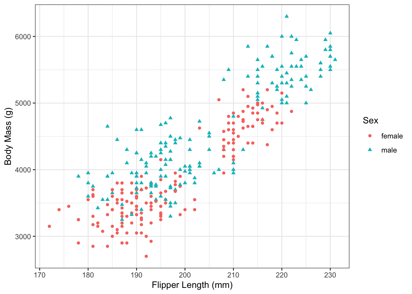
Figure 8.1: Flipper length and body mass in the Palmer Penguin dataset.
Let’s use the following notation for modeling the penguin data:
- \(Y_i =\) Body mass (in grams) for penguin \(i\)
- \(x_{i1} =\) Flipper length (in mm) for penguin \(i\)
- \(x_{i2} =\) Indicator of sex for penguin \(i\). Set \(x_{i2}= 0\) for female penguins and \(x_{i2}=1\) for male penguins.
The MLR model for these data are:
\[\begin{equation} Y_i = \beta_0 + \beta_1x_{i1} + \beta_2x_{i2} + \epsilon_i \tag{8.2} \end{equation}\]
Because the variable for sex has only two possible values (0 and 1), we can construct two different regression lines from equation (8.2). For female penguins, \(x_{i2} = 0\), so (8.2) reduces to:
\[\begin{align} Y_i &= \beta_0 + \beta_1x_{i1} + \beta_2(0) + \epsilon_i\\ &= \beta_0 + \beta_1x_{i1} + \epsilon_i \tag{8.3} \end{align}\]
Notice that this equation looks almost exactly like an SLR model. To interpret \(\beta_0\) and \(\beta_1\) in (8.3), it is helpful to calculate the expected value of \(Y\) to find the regression line for mean body mass of female penguins:
\[\begin{equation} \E[Y_i | x_{i1} = x_{i1}, x_{i2} = 0] = \beta_0 + \beta_1x_{i1} \tag{8.4} \end{equation}\]
Notice here how we are using the notation \(\E[Y_i | x_{i1} = x_{i1}, x_{i2} = 0]\) to denote the expected value of \(Y_i\) for observations with \(x_{i1} = x_{i1}\) and \(x_{i2} = 0\). This is an example of general notation for the expectation of \(Y\) conditional on specific values of the predictor variables \(x_{ij}\). Equation (8.4) tells us that the average flipper length of female penguins is \(\beta_0\) plus \(\beta_1\) times the flipper length–exactly the kind of interpretation we saw in SLR>
For male penguins, \(x_{i2} = 0\), so equation (8.2) reduces to: \[\begin{align} Y_i &= \beta_0 + \beta_1x_{i1} + \beta_2(1) + \epsilon_i\\ &= (\beta_0 + \beta_2) + \beta_1x_{i1} + \epsilon_i \tag{8.5} \end{align}\] Notice that in the second line of (8.5), we have grouped \(\beta_0\) and \(\beta_2\) together. This is because in (8.5), the sum of these parameters functions as the intercept of the model. Taking the expectation of (8.5) gives the equation for the regression line for mean body mass of male penguins: \[\begin{equation} \E[Y_i| x_{i1} = x_{i1}, x_{i2} = 1] = (\beta_0 + \beta_2) + \beta_1x_{i1} \tag{8.6} \end{equation}\]
The key difference between equations (8.4) and (8.6) is in the intercept. For female penguins, the intercept of the line is \(\beta_0\), while for male penguins it is \(\beta_0 + \beta_2\). Both lines still have the same slope, \(\beta_1\). We can plot these equations over the data to graphically represent the model:
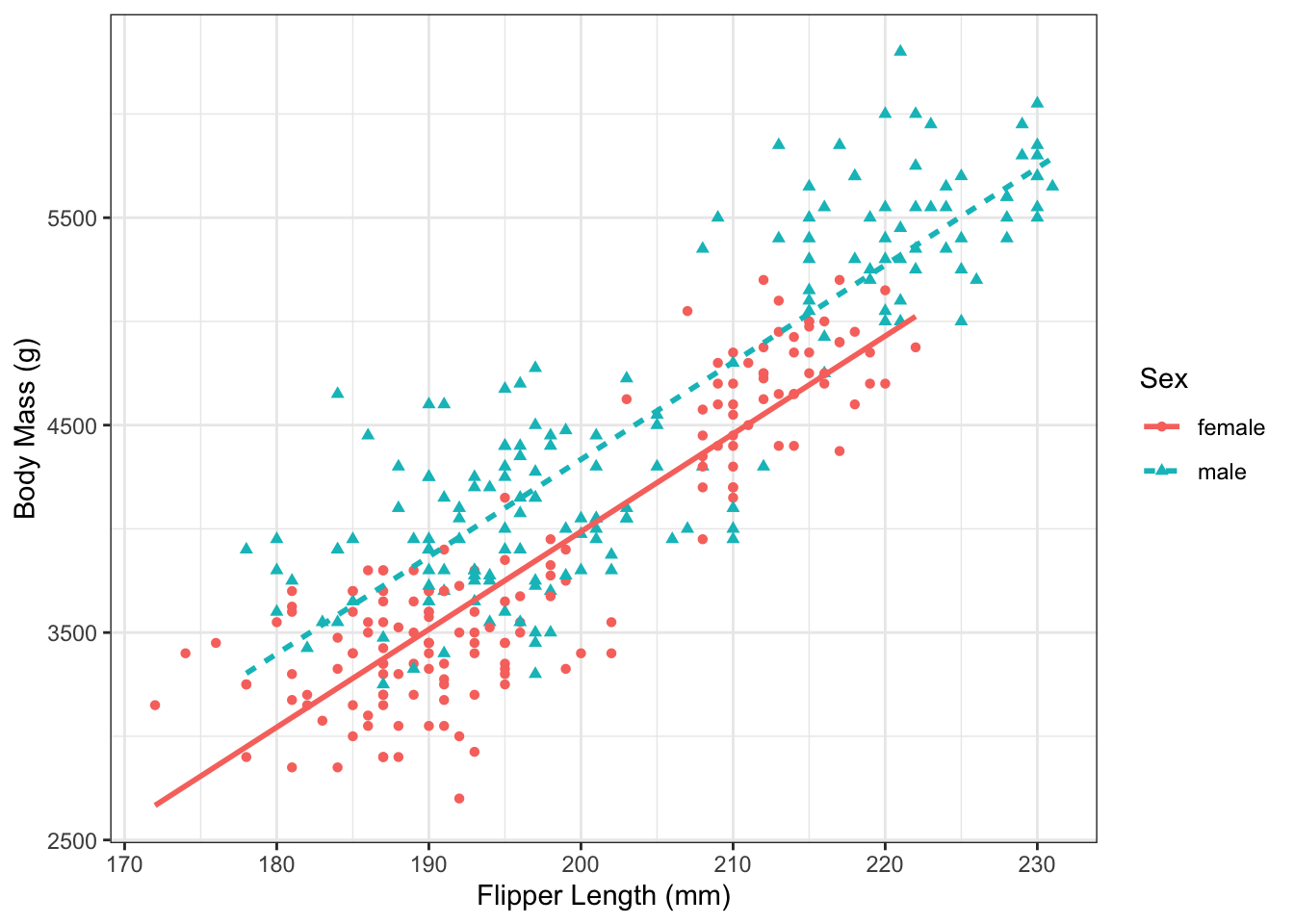
Figure 8.2: Flipper length and body mass in the Palmer Penguin dataset.
Comparing the mean body mass of penguins of the same sex, but with different flipper lengths, amounts to comparing different points along one of the lines in Figure 8.2. Meanwhile, comparing the mean body mass of penguins with the same flipper length, but of different sexes, amounts to comparing values vertically between the lines. Example 8.1 lays this out in more detail.
Example 8.1 Consider the following groups of penguins:
- Group A: Female penguins with 200mm flippers
- Group B: Female penguins with 190mm flippers
- Group C: Male penguins with 200mm flippers
- Group D: Male penguins with 190mm flippers
Part 1: According to the MLR model (8.2), what is the difference in average body mass between penguins in Group A and Group B?
To answer this, let’s first write out the equation of the mean body mass for each group of penguins: \[\text{Group A:} \quad \E[Y_i | x_{i1} = 200, x_{i2} = 0 ] = \beta_0 + \beta_1*200\] \[\text{Group B:} \quad \E[Y_i | x_{i1} = 190, x_{i2} = 0 ] = \beta_0 + \beta_1*190\] The difference between these is: \[\begin{align*} \E[Y_i | x_{i1} = 200, x_{i2} = 0 ] - \E[Y_i | x_{i1} = 190, x_{i2} = 0 ] &= \left(\beta_0 + \beta_1*200 \right) - \left(\beta_0 + \beta_1*190\right)\\ & = 200\beta_1 - 190\beta_1\\ &= 10\beta_1 \end{align*}\] So for female penguins that differ in flipper length by 10mm, the difference in their average body mass is \(10\beta_1\).
Part 2: According to the MLR model (8.2), what is the difference in average body mass between penguins in Group C and Group D?
We follow the same procedure, first finding the equation for the mean body mass in each group and then computing their difference. \[\text{Group C:} \quad \E[Y_i | x_{i1} = 200, x_{i2} = 1 ] = \beta_0 + \beta_2 + \beta_1*200\] \[\text{Group D:} \quad \E[Y_i | x_{i1} = 190, x_{i2} = 1 ] = \beta_0 + \beta_2 + \beta_1*190\]
\[\begin{align*} \E[Y_i | x_{i1} = 200, x_{i2} = 1 ] - \E[Y_i | x_{i1} = 190, x_{i2} = 1 ] &= \left(\beta_0 + \beta_2 + \beta_1*200 \right)\\ & \quad - \left(\beta_0 + \beta_2 + \beta_1*190\right)\\ & = 200\beta_1 - 190\beta_1\\ &= 10\beta_1 \end{align*}\] So for male penguins that differ in flipper length by 10mm, the difference in their average body mass is \(10\beta_1\).
Part 3: According to the MLR model (8.2), what is the difference in average body mass between penguins in Group C and Group A?
\[\begin{align*} \E[Y_i | x_{i1} = 200, x_{i2} = 1 ] - \E[Y_i | x_{i1} = 200, x_{i2} = 0 ] &= \left(\beta_0 + \beta_2 + \beta_1*200 \right)\\ & \quad - \left(\beta_0 + \beta_2 + \beta_1*200\right)\\ & = \beta_2 \end{align*}\] We would obtain the same difference if we compared Group D to Group B. So for penguins with the same flipper length, the difference in body mass between male penguins and female penguins is \(\beta_2\).
8.3 MLR Model 2: Two continuous predictors
Instead of modelling body mass using flipper length and sex, we could instead model body mass using flipper length and bill length. Mathematically, this means considering a model with two continuous predictor variables.
First, we can graphically see that there appears to be a positive correlation between bill depth, flipper length, and body mass.

We can again use equation (8.2) as our model, but now the variables are:
- \(Y_i =\) Body mass (in grams) for penguin \(i\)
- \(x_{i1} =\) Flipper length (in mm) for penguin \(i\)
- \(x_{i2} =\) Bill length (in mm) for penguin \(i\)
This setting is more complex than the one in Section 8.2, because \(x_{i2}\) could take on any value and not just 0/1. This means that we can’t easily plot all of the relationships like in Figure 8.2. However, we can still apply an algebraic approach to understand what each parameter represents.
Example 8.2 What is the difference in average body mass for penguins with the same flipper length and that differ in bill length by 1 mm?
In this example, we don’t know the specific flipper length of the penguins, but we are told that they have the same length. So when computing their mean body mass, we can use a variable (\(x_1\)) to represent this value. We also don’t know what their bill depths are, except that they differ by one unit. We can use \(x_2 + 1\) and \(x_2\) to denote these two quantities. The difference in average body mass between the specified groups of penguins is:
\[\begin{align*} \E[Y_i | x_{i1} = x_1, x_{i2} = x_2 + 1 ] \qquad &\\ - \E[Y_i | x_{i1} = x_1, x_{i2} = x_2 ] &= \left(\beta_0 + \beta_1*x_1 + \beta_2(x_2 + 1)\right) - \left(\beta_0 + \beta_1*x_1 + \beta_2x_2\right)\\ & = (x_2 + 1)\beta_2 - x_2\beta_2\\ &= \beta_2 \end{align*}\]
By the same procedure, we could find that the difference in average body mass for penguins with the same bill length that differ in flipper length by 1mm is \(\beta_1\).
8.4 Interpreting \(\beta_j\) in the general MLR model
The examples above show us that for the MLR model with two predictor variables, the coefficient parameters can be interpreted as:
- \(\beta_0 =\) Average value of \(Y_i\) for observations with \(x_{i1}=0\) and \(x_{i2}=0\)
- \(\beta_1 =\) Difference in average value of \(Y_i\) for a 1-unit difference in \(x_{i1}\) among observations with the same value of \(x_{i2}\)
- \(\beta_2 =\) Difference in average value of \(Y_i\) for a 1-unit difference in \(x_{i2}\) among observations with the same value of \(x_{i1}\)
The key part to these interpretations is that we are comparing differences in the outcome when the other variable is held constant. This generalizes to models with more predictor variables as follows:
- \(\beta_0 =\) Average value of \(Y_i\) when all the \(x\)’s are zero
- \(\beta_j =\) Average difference in \(Y_i\) for a 1-unit difference in \(x_{ij}\) among observations with the same value of all other \(x\)’s
There are cases where we need to be extra careful in interpreting the coefficients, particularly when multiple predictor variables are related to one another. We will see examples of this in Sections 11 and 14.
8.5 Linear Combinations of \(\beta_j\)’s
In multiple linear regression, it is common to compare observations that differ in more than one predictor variable and to compute the mean value of the outcome for a specified combination of predictor variables. Both of these use a linear combination of the \(\beta\)’s to calculate means and compare values.
8.5.1 Computing Mean Values
To compute the mean value for a combination of predictor variables, we simply plug those values into the MLR equation. The average value of \(Y\) for an observation with \(x_{i1} =a_1\), \(x_{i2} = a_2\), , \(x_{ik}=a_{ik}\) is \[\E[Y_i | x_{i1}=a_1, \dots, x_{ik} = a_k] = \beta_0 +a_1\beta_1 + \dots + a_k\beta_k\] Since we are computing the mean value, the equation on the right-hand side includes the intercept \(\beta_0\).
Example 8.3 Consider an MLR model for penguin body mass that includes three predictors: flipper length (\(x_1\)), bill length (\(x_2\)), and sex (\(x_3\) is indicator of being male). What is the mean body mass for male penguins with flipper lengths of 200 mm, bill lengths of 45 mm?
To answer this, we plug in \(x_1 = 200\), \(x_2 = 45\), and \(x_3 = 1\) to get the mean value \[E[Y] = \beta_0 + 200\beta_1 + 45\beta_2 + \beta_3\]
8.5.2 Computing Differences
To find the difference in mean value of the outcome between two observations with different predictor variable values, we can compute the mean for each and subtract.
Example 8.4 Use the MLR model from Example 8.3 to find the difference in mean body mass between female penguins with 150 mm flippers and 45 mm bills and male penguins with 200 mm flippers and 38 mm bills.
Solution. We start with finding the mean for each: \[E[Y | x_1 = 150, x_2 = 45, x_3 = 0] = \beta_0 + 150\beta_1 + 45\beta_2\] \[E[Y | x_1 = 200, x_2 = 38, x_3 = 1] = \beta_0 + 200\beta_1 + 38\beta_2 + \beta_3\] Taking the difference, we find: \[E[Y | x_1 = 150, x_2 = 45, x_3 = 0] - E[Y | x_1 = 200, x_2 = 38, x_3 = 1] = -50\beta_1 + 9 \beta_2 - \beta_3\]
Generalizing the result from Example 8.4, we can interpret the value of \[a_1\beta_1 + a_2\beta_2 + \dots + a_k\beta_k\] as the difference in the expected value of the outcome between observations that differ by \(a_1\) in \(x_1\), \(a_2\) in \(x_2\),\(\dots\), and \(a_k\) in \(x_k\).
It’s important to keep in mind that if we are given a linear combination of \(\beta\)’s that does include \(\beta_0\), then it represents a mean value. And if it does not include \(\beta_0\), then it represents a difference in means.
8.6 Exercises
Exercise 8.1 Suppose we have data on several football teams, with one observation per team for a set of games in the football season. We fit an MLR model with the variables:
- \(Y_i\) = Points scored
- \(x_{i1}\) = Rushing yards
- \(x_{i2}\) = Passing yards
- \(x_{i3}\) = Number of turnovers
In the context of this model, provide an interpretation for each of the following:
- \(150\beta_1\)
- \(200\beta_2 + 3\beta_3\)
- \(-\beta_3\)
- \(\beta_0 + 100\beta_1 + 150\beta_2\)
- \(\beta_0\)
Exercise 8.2 Using the model from Exercise 8.1, find the following values in terms of \(\beta\)’s:
- The mean number of points scored for a team that had 130 rushing yards, 75 passing yards, and 2 turnovers.
- The difference in mean number of points scored, comparing a team with 230 passing yards, and 1 turnover to a team with 300 passing yards, 50 rushing yards, and 3 turnovers.
- The difference in mean number of points scored between two teams that differ in passing yards by 50 but have the same mnumber of rushing yards and turnovers.
- The difference in mean number of points scored between two teams that differ in rushing yards by 25 and turnovers by 4 but have the same mnumber of passing yards.
- The difference in mean number of points scored, comparing a team with 300 passing yards, 50 rushing yards, and 3 turnover to a team with 230 passing yards, 100 rushing yards, and 1 turnovers. (Hint: Can you calculate this directly from your answer to (b)?)