Chapter 4 Inference on \(\beta\) in SLR
\(\newcommand{\E}{\mathrm{E}}\) \(\newcommand{\Var}{\mathrm{Var}}\) \(\newcommand{\bmx}{\mathbf{x}}\) \(\newcommand{\bmX}{\mathbf{X}}\)
4.1 Inference Goals
A fundamental task in statistics is inference, in which we use a sample of data to make generalizations about relationships in larger populations. Inference is a key component of an association analysis (see Section 1.2.1). Inference is usually conducted via hypothesis tests and confidence intervals.
Statistical inference is rooted in an underlying scientific goal. A standard inferential question for a regression analysis is something like: Is there a relationship between ‘x’ and the average value of ‘y’?, where ‘x’ and ‘y’ are a predictor and outcome of interest. To answer this question using regression, we first need to translate it into a statistical question about specific model parameters.
It helps to first note that if there is no relationship between the variable \(x\) and the average outcome \(\E[Y]\), then an appropriate linear model is the intercept-only model:
\[\begin{equation} Y_i = \beta_0 + \epsilon_i. \tag{4.1} \end{equation}\] In equation (4.1), the predictor \(x\) does not appear at all, and so the regression line is simply a horizontal line with intercept \(\beta_0\). Figure 4.1 shows an example of data generated from a model in which there is no relationship between \(Y_i\) and \(x_i\).
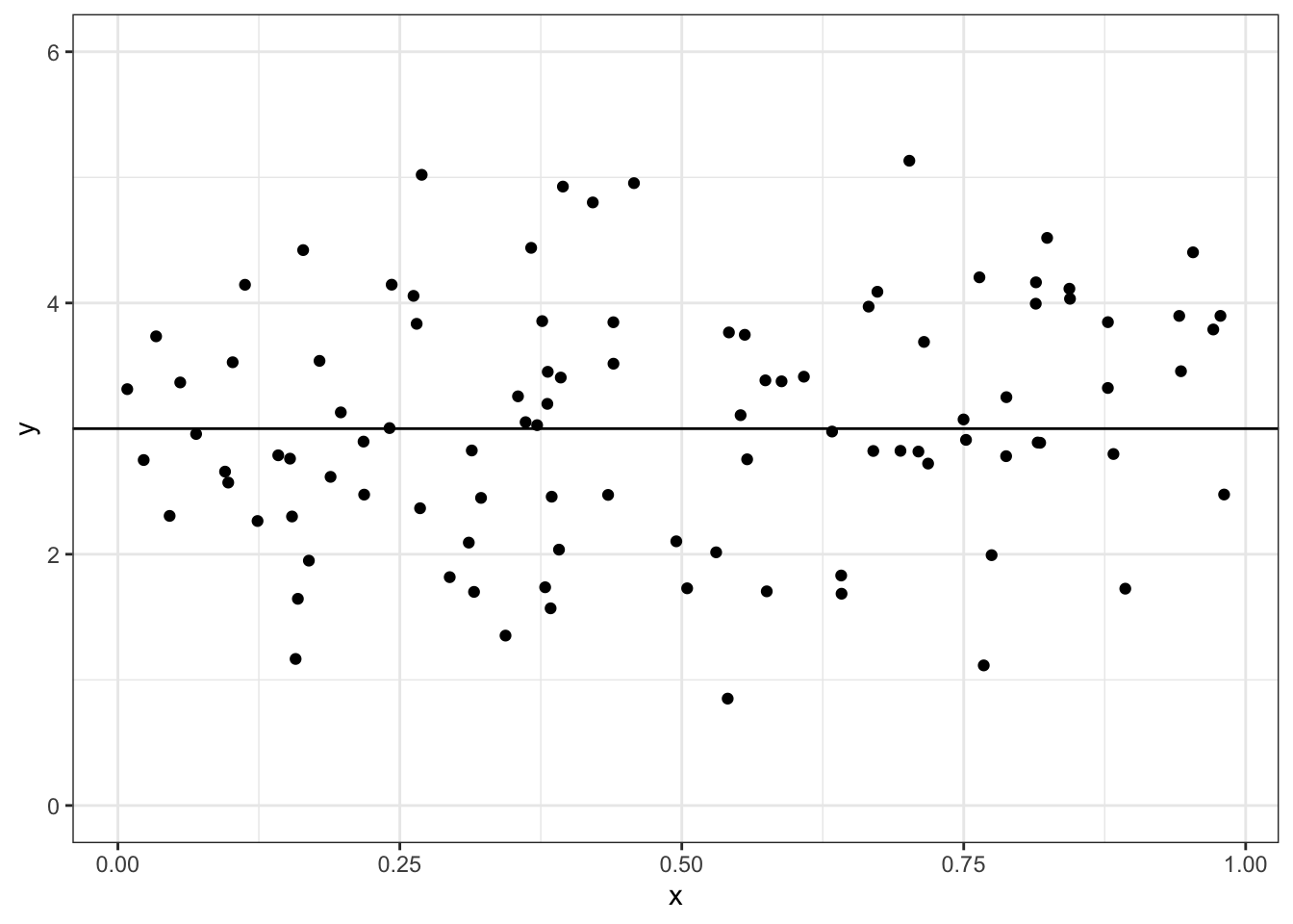
Figure 4.1: Example data from a hypothetical regression model with \(\beta_0 = 3\) and \(\beta_1 = 0\). The black line shows the true mean of \(y\) as a function of \(x\).
How is the intercept-only model useful? Well, it allows to change the scientific question:
Is there a relationship between ‘x’ and the average value of ‘y’?
into a statistical question:
In the model \(Y_i = \beta_0 + \beta_1x_i + \epsilon_i\), is \(\beta_1 \ne 0\)?
If the answer to this question is “No”, then \(\beta_1 = 0\) and we are left with the intercept-only model.
Example 4.1 In the penguin data we might ask: Is there a relationship between flipper length and body mass in penguins? The corresponding statistical question is: In the SLR model with \(x_i =\) flipper length and \(Y_i =\) body mass, is \(\beta_1 \ne 0\)? We saw in Example ?? that the estimated SLR equation for the penguin data was \(\E[Y_i] = -5780.83 + 49.69x_i\). Thus, the estimated slope is 49.7 g/mm. Clearly this value is not 0. But is it meaningfully different from 0? We address that question in the remainder of this chapter.
4.2 Standard Error of \(\beta_1\)
4.2.1 Sampling Distribution of \(\hat\beta_1\)
The notation \(\hat\beta_1\) actually refers to two different quantities. On one hand, this is the estimated slope of the linear regression line; that is, \(\hat\beta_1\) is a number or an estimate. But \(\hat\beta_1 = S_{xy}/S_{xx}\) also denotes an estimator, which is a rule for calculating an estimate from a dataset.
As an estimator, \(\hat\beta_1\) has a distribution. We have previously seen that under the standard SLR assumptions:
- \(\E[\hat\beta_1] = \beta_1\)
- \(\Var[\hat\beta_1] =\sigma^2/S_{xx}\)
The value of \(\Var[\hat\beta_1]\) tells about how much variation there is the values of \(\hat\beta_1\) calculated from many different datasets. If we conduct repeated experiments all using the same population and settings, we obtain a different \(\hat\beta_1\) each time.
- The distribution of values we obtain is called the of \(\hat\beta_1\)
- The standard deviation (or the variance) of this distribution tells us about the uncertainty in \(\hat\beta_1\)
4.2.2 Standard Errors
The standard deviation of the sampling distribution of \(\hat\beta_1\) is called the standard error of \(\hat\beta_1\) and it is denoted:
\[se(\hat\beta_1) = \sqrt{\Var(\hat\beta_1)} = \sqrt{\sigma^2/S_{xx}}\] The value of \(se(\hat\beta_1)\) depends on three factors:
- The variance of the error terms (\(\sigma^2\))
- The variation in the values of \(x_i\) (via \(S_{xx}\))
- The number of observations (via \(S_{xx}\))
It’s important to note that we don’t know \(\sigma^2\), but we can estimate it as \(\hat\sigma^2\) (see Section 3.4.3). This gives an estimate of \(\Var(\hat\beta_1)\): \[\widehat{\Var}(\hat\beta_1) = \dfrac{\hat\sigma^2}{S_{xx}} = \dfrac{1}{S_{xx}}\dfrac{1}{n-2}\sum_{i=1}^n e_i^2\] So we calculate the estimated standard error as \[\widehat{se}(\hat\beta_1) = \sqrt{\dfrac{MS_{res}}{S_{xx}}}\]
4.3 Not Regression: One-sample \(t\)-test
To see how we incorporate \(se(\hat\beta_1)\) into a hypothesis test, let’s first go back to perhaps the most well-known test in statistics, the one-sample \(t\)-test.
For a one-sample \(t\)-test, we assume that we have an independent sample of values \(y_1\), \(y_2\), \(\dots\), \(y_n\) from a population in which \(Y_i \sim N(\mu, \sigma^2)\). Our hypothesis is then to test whether \(\mu \ne \mu_0\) for some chosen value of \(\mu_0\). We can write this as: \[H_0: \mu = \mu_0 \quad \text{vs.} \quad H_A: \mu \ne \mu_0\] We use the test statistic \[t = \frac{\hat\mu - \mu_0}{se(\hat\mu)}.\] If \(H_0\) is true, then \(t\) follows a \(T\)-distribution with \(n-1\) degrees of freedom, i.e. \(t \sim T_{(n-1)}\).
- If \(t\) is “large”, then we reject \(H_0\) in favor of \(H_A\)
- If \(t\) is not “large”, then we do not reject \(H_0\)
But what does “large” value of \(t\) mean? Large \(t\) means \(\overline{y}\) is far from the hypothesized value \(\mu_0\). To account for the variability in the distribution of \(\hat\beta_1\), we divide \(\overline{y} - \mu_0\) by its standard error. This is because a large difference between \(\overline{y}\) and \(\mu_0\) is more meaningful when \(\overline{y}\) has smaller variance.
We then compare \(t\) to the \(T_{n-1}\) distribution and compute \(P(T > |t|)\):
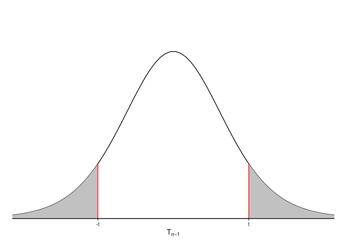
Figure 4.2: Density curve for T-distribution. Shaded areas on left and right represent \(P(T > |t|)\).
This probability is given by the shaded areas on the right and left in Figure 4.2. Since our alternative hypothesis is two-sided (as opposed to a one-sided hypothesis such as \(H_0: \mu > \mu_0\)), then we need to consider the values in both directions.
If \(p=P(T > |t|)\) (the “\(p\)-value”) is smaller than the chosen critical value \(\alpha\), then we reject \(H_0\). How to choose \(\alpha\) is the subject of much debate, but a widely used value is 0.05. In some contexts, 0.01 and 0.1 are also used as critical values for rejecting \(H_0\).
If \(P(T > |t|) > \alpha\), then we fail to reject \(H_0\). It’s important to note that failing to reject \(H_0\) is not the same as proving \(H_0\)!
Why is \(t \sim T_{n-1}\) and not \(t \sim N(0, 1)\)? This is because we have estimated the standard error \(\widehat{se}(\overline{y}) = s/\sqrt{n}\), and so \(t\) has more variation than a normal distribution. Part of what makes tests of this form so useful is that when \(n\) (the sample size) is large enough, then \(t\) has a \(T\)-distribution, even if \(Y\) does not have a normal distribution! This is a consequence of the Central Limit Theorem (CLT).
The CLT tells us that for a sequence of random variables \(X_1\), \(X_2\), with finite mean \(\mu\) and finite variance \(\sigma^2\), the distribution of the mean of the observations \(\overline{X}_n = \frac{1}{n}\sum_{i=1}^n X_i\) can be approximated by a normal distribution with mean \(\mu\) and variance \(\sigma^2/n\) when \(n\) is sufficiently large.
4.4 \(p\)-values
While widely used, \(p\)-values are commonly mis-used. It’s important to keep in mind what a \(p\)-value can (and can’t!) tell you. A formal definition for a \(p\)-value is:
Definition 4.1 The \(p\)-value for a hypothesis test is the probability, if \(H_0\) is true, of observing a test statistic the same or more in favor of the alternative hypothesis than the result that was obtained.
The underlying idea is that a small \(p\)-value means that getting data like what we observed is not very compatible with \(H_0\) being true.
Incorrect interpretations of \(p\)-values:
- Probability the null hypothesis is incorrect
- Probability that the alternative hypothesis is true
- Probability of these results occurring by chance
In 2018, the American Statistical Association (ASA) published a statement about \(p\)-values.1 Included in that statement were the following reminders:
- \(p\)-values can indicate how incompatible the data are with a specified statistical model.
- \(p\)-values do not measure the probability that the studied hypothesis is true, or the probability that the data were produced by random chance alone.
- Scientific conclusions and business or policy decisions should not be based only on whether a \(p\)-value passes a specific threshold.
- Proper inference requires full reporting and transparency.
- A \(p\)-value, or statistical significance, does not measure the size of an effect or the importance of a result.
- By itself, a \(p\)-value does not provide a good measure of evidence regarding a model or hypothesis.
4.5 Hypothesis Testing for \(\beta_1\)
In simple linear regression, we can conduct a hypothesis test for \(\beta_1\) just like how we conducted the one-sample \(t\)-test.
First, we set up the null and alternative hypotheses:
\(H_0: \beta_1 = \beta_{10}\) \(H_A: \beta_1 \ne \beta_{10}\)2
Most commonly, \(\beta_{10} = 0\), which mean we are testing whether there is a relationship between \(x\) and \(\E[Y]\). The \(t\) statistic is:
\[t = \dfrac{\hat\beta_1 - \beta_{10}}{\widehat{se}(\hat\beta_1)} = \dfrac{\hat\beta_1 - \beta_{10}}{\sqrt{\hat\sigma^2/S_{xx}}} = \dfrac{\hat\beta_1 - \beta_{10}}{\sqrt{\frac{1}{S_{xx}}\frac{1}{n-2}\sum_{i=1}^ne_i^2}}\]
If \(\epsilon_i \sim N(0, \sigma^2)\) and \(H_0\) is true, then \(t\) has a \(T\)-distribution with \(n-2\) degrees of freedom. If \(H_0\) is true, but \(\epsilon_i\) is not normally distributed, then \(t\) follows a \(T_{n-2}\) distribution approximately, because of the CLT. We reject \(H_0\) at the \(\alpha\) level if \(P(T > |t|) < \alpha\).
Example 4.2 Let’s return to the penguin data in Example 4.1, in which we asked: In the SLR model with \(x_i =\) flipper length and \(Y_i =\) body mass, is \(\beta_1 \ne 0\)?
We previously calculated the estimated slope as \(\hat\beta_1 = 49.7\). From the question formulation, we know that the test value \(\beta_{10} = 0\). To calculate \(t\), we now need to compute \(\widehat{se}(\hat\beta_1) = \hat\sigma^2/S_{xx}\).
We can obtain \(\hat\sigma^2\) from R, either from the output of summary() or by calculating it directly:
penguin_lm <- lm(body_mass_g ~ flipper_length_mm, data=penguins)
sig2hat <- summary(penguin_lm)$sigma^2
sig2hat
## [1] 155455.3## [1] 155455.3We can then calculate \(S_{xx}\) as:
sxx <- sum(penguins$flipper_length_mm^2, na.rm=T) - 1/nobs(penguin_lm)*sum(penguins$flipper_length_mm, na.rm=T)^2
sxx
## [1] 67426.54Now we combine these values to compute
\[t = \frac{\hat\beta_1 - \beta_{10}}{\sqrt{\hat\sigma^2/S_{xx}}} = \frac{49.7 - 0}{\sqrt{155455.3/67426.54}} = 32.7\] In R, this computation is:
## flipper_length_mm
##          32.72223
We can then compute the \(p\)-value, by comparing to a \(T\)-distribution:
## flipper_length_mm
##     4.370681e-107
This tell us that \(P(T > |32.7|) < 0.0001\). And so we reject \(H_0\) at the \(\alpha = 0.001\) level.
Although the method just describe works, it can be tedious and is prone to mistakes. Since the null hypothesis \(H_0: \beta_1 = 0\) is so commonly tested, R provides the results of the corresponding hypothesis test in its standard output.
Example 4.3 Compare the following output with the results calculated manually in Example 4.2.
## # A tibble: 2 × 5
##   term              estimate std.error statistic   p.value
##   <chr>                <dbl>     <dbl>     <dbl>     <dbl>
## 1 (Intercept)        -5781.     306.       -18.9 5.59e- 55
## 2 flipper_length_mm     49.7      1.52      32.7 4.37e-107
We see a column with \(\hat\beta_1\), \(\widehat{se}(\hat\beta_1)\), \(t\), and \(p\)! This same information is also available from the summmary() command:
##
## Call:
## lm(formula = body_mass_g ~ flipper_length_mm, data = penguins)
##
## Residuals:
##      Min       1Q   Median       3Q      Max
## -1058.80  -259.27   -26.88   247.33  1288.69
##
## Coefficients:
##                    Estimate Std. Error t value Pr(>|t|)
## (Intercept)       -5780.831    305.815  -18.90   <2e-16 ***
## flipper_length_mm    49.686      1.518   32.72   <2e-16 ***
## ---
## Signif. codes:  0 '***' 0.001 '**' 0.01 '*' 0.05 '.' 0.1 ' ' 1
##
## Residual standard error: 394.3 on 340 degrees of freedom
##   (2 observations deleted due to missingness)
## Multiple R-squared:  0.759,  Adjusted R-squared:  0.7583
## F-statistic:  1071 on 1 and 340 DF,  p-value: < 2.2e-16
4.6 Other forms of hypothesis tests for \(\beta_1\)
4.6.1 Testing against values other than 0
Although less common, it is possible to conduct hypothesis tests against a null value other than zero. For example, we could set up the hypotheses
\[\begin{equation} H_0 : \beta_1 = 40 \quad \text{vs.} \quad H_A: \beta_1 \ne 40 \tag{4.2} \end{equation}\]
To conduct this hypothesis test, we would need to use the “by hand” procedure for computing \(t\) and \(p\).
Example 4.4 In the penguin data from Example 4.1, what is the conclusion of testing the null hypothesis in Equation (4.2)?
We compute \(t\) as:
\[t = \frac{49.7 - 40}{1.52} = 6.38\]
In R, this can be computed as:
## [1] 6.378781We can then compute the \(p\)-value, by comparing to a \(T\)-distribution:
## [1] 5.832893e-10We reject the null hypothesis that \(\beta_1 = 40\) at the \(\alpha < 0.0001\) level.
4.6.2 One-sided tests
Another alternative is a one-sided test, which involves null and alternative hypotheses of the form:
\[\begin{equation} H_0 : \beta_1 \ge 0 \quad \text{vs.} \quad H_A: \beta_1 < 0 \tag{4.2} \end{equation}\]
With one-sided hypotheses, the calculation of \(t\) is the same as in the two-sided setting, but the calculation of the \(p\)-value is different. Instead of \(p = P(T > |t|)\), we evaluate \(p = P(T > t)\) or \(P(T < p)\), depending on whether the alternative hypothesis is greater than (\(>\)) or less than (\(<\)). The direction of the inequality for calculating the \(p\)-value should always match the direction in the alternative hypothesis.
Example 4.5 In the penguin data from Example 4.1, what is the conclusion from a test of the hypotheses in equation (4.2)?
We can use the value \(t=32.7\) calculated earlier. But now we evaluated the \(p\)-value as:
## [1] 1In this example, \(p \approx 1\), so we fail to reject the null hypothesis that \(\beta_1\) is greater than or equal to zero. This should come as no surprise, since our estimate \(\hat\beta_1\) is (much) greater than zero.
4.7 Confidence Intervals (CIs)
4.7.1 Definition and Interpretation
Hypothesis tests provide an answer to a specific question (Is there evidence to reject the null hypothesis?), but they don’t directly provide information about the uncertainty in the point estimates. In many contexts, what is often more useful than a conclusion from a hypothesis test is an estimate of a parameter and its uncertainty. Confidence intervals provide a way to describe the uncertainty in a parameter estimate.
Definition 4.2 A \((1- \alpha)100\%\) confidence interval is a random interval that, if the model is correct, would include (“cover”) the true value of the parameter with probability \((1 - \alpha)\).
In this definition, it is important to note that the interval is random, not the parameter. The parameter is a fixed, but unknown, constant, and so it cannot have a probability distribution associated with it.3 A common incorrect interpretation of a CI is that the probability of the parameter being in the interval is \((1- \alpha)100\%\).
For a single dataset, there is no guarantee that the true value of a parameter will be included within the confidence interval. But if the model is correct, then an interval generated by the same procedure should include the true value in \((1-\alpha)100\%\) of analysis of independently-collected data. Figure 4.3 shows the coverage of 95% CIs calculated for 100 simulated datasets when the true value of \(\beta_1 = 2\).
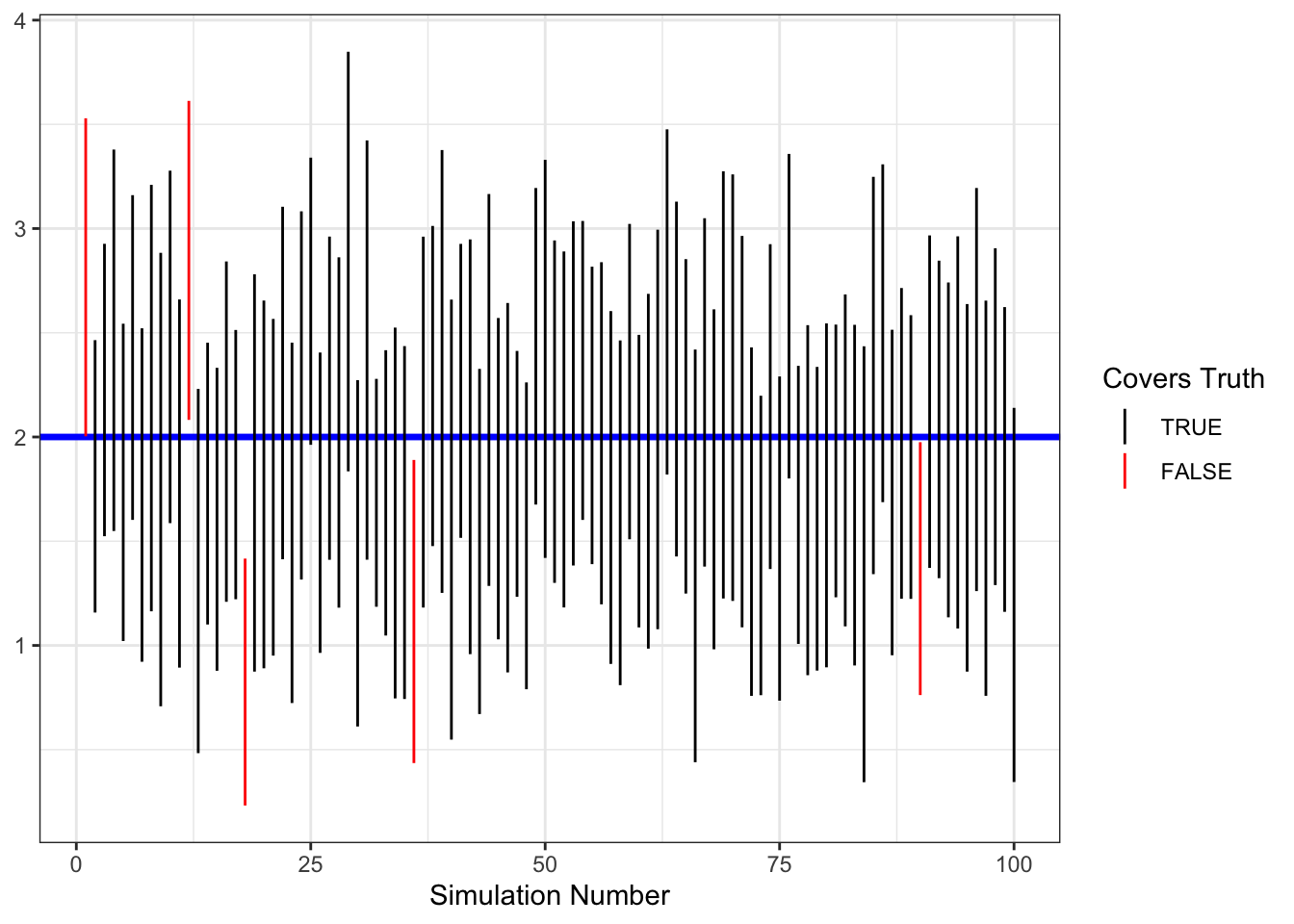
Figure 4.3: Example of coverage of 95% CIs in 100 simulated datasets.
4.7.2 Inverting a Hypothesis Test
To create a confidence interval, we invert a hypothesis test. Recall that for testing the null hypothesis \(H_0: \beta_1 = \beta_{10}\) against the alternative hypothesis \(H_A: \beta_1 \ne \beta_{10}\), we computed the test statistic \[t = \frac{\hat\beta_1 - \beta_{10}}{\widehat{se}(\hat\beta_1)}\] by plugging in \(\hat\beta_1\), \(\widehat{se}(\hat\beta_1)\), and \(\beta_{10}\). We then compared the value of \(t\) to a \(T_{n-2}\) distribution to compute the \(p\)-value \(p=P(T > |t|)\). For a confidence interval, we reverse this process. That is, we plug in \(\hat\beta_1\), \(\widehat{se}(\hat\beta_1)\), and \(t\), then solve for \(\beta_{10}\) as an unknown value.
The distribution of \(t = \dfrac{\hat\beta_1 - \beta_{1}}{\widehat{se}(\hat\beta_1)}\) is \(T_{n-2}\). This distribution has mean zero and a standardized variance (it’s close to 1, although not exactly 1). There exists a number, which we denote \(t_{\alpha/2}\), such that the area under the curve between \(-t_{\alpha/2}\) and \(t_{\alpha/2}\) is \(1-\alpha\). Mathematically, this can be written:
\[\begin{equation} P\left(-t_{\alpha/2} \le \dfrac{\hat\beta_1 - \beta_1}{\widehat{se}(\hat\beta_1)} \le t_{\alpha/2}\right) = 1 - \alpha \tag{4.3} \end{equation}\]
Graphically, this looks like:

We can rearrange equation (4.3), so that \(\beta_1\) is alone in the middle:
\[\begin{align*} 1-\alpha &= P\left(-t_{\alpha/2}\widehat{se}(\hat\beta_1) \le \hat\beta_1 - \beta_1 \le t_{\alpha/2}\widehat{se}(\hat\beta_1)\right)\\ &= P\left(t_{\alpha/2}\widehat{se}(\hat\beta_1) \ge \beta_1 - \hat\beta_1 \ge -t_{\alpha/2}\widehat{se}(\hat\beta_1)\right)\\ &= P\left(\hat\beta_1 + t_{\alpha/2}\widehat{se}(\hat\beta_1) \ge \beta_1 \ge \hat\beta_1 -t_{\alpha/2}\widehat{se}(\hat\beta_1)\right)\\ &= P\left(\hat\beta_1 - t_{\alpha/2}\widehat{se}(\hat\beta_1) \le \beta_1 \le \hat\beta_1 + t_{\alpha/2}\widehat{se}(\hat\beta_1)\right)\\ \end{align*}\]
4.8 CIs for \(\beta_1\)
The procedure from the previous section gives a \((1 -\alpha)100\%\) confidence interval for \(\beta_1\): \[\left(\hat\beta_1 - t_{\alpha/2}\widehat{se}(\hat\beta_1), \hat\beta_1 + t_{\alpha/2}\widehat{se}(\hat\beta_1)\right)\]
4.8.1 Confidence Intervals “by hand” in R
To compute a confidence interval “by hand” in R, we can plug in the appropriate values into the formulas. The estimates \(\hat\beta_1\) and \(\widehat{se}(\hat\beta_1)\) can be calculated from an lm object.
To compute \(t_{\alpha/2}\), use the qt() command, which can be used to find \(x\) such that \(P(T < x) = \tilde{p}\) for a given value of \(\tilde{p}\).
In order to compute \(t_{\alpha/2}\), we need to find \(x\) such that \(P(T < x) = 1- \alpha/2\).
Because of the symmetry of the \(T\) distribution, this will yield an \(x = t_{\alpha/2}\).
This can be implemented in the following code:
## [1] 1.984467An alternative approach is to find \(P(T > x ) = \alpha/2\). To do this using qt(), set the lower=FALSE option:
## [1] 1.984467Example 4.6 In the penguin data, suppose we wish to construct a confidence interval for \(\beta_1\) using the formulas. This can be done with the following code:
penguin_lm <- lm(body_mass_g~flipper_length_mm,
                data=penguins)
alpha <- 0.05
t_alphaOver2 <- qt(1-alpha/2,
                   df = nobs(penguin_lm)-2)
CI95Lower <- coef(penguin_lm)[2] - t_alphaOver2 * tidy(penguin_lm)$std.error[2]
CI95Upper <- coef(penguin_lm)[2] + t_alphaOver2 * tidy(penguin_lm)$std.error[2]
c(CI95Lower, CI95Upper)
## flipper_length_mm flipper_length_mm
## 46.69892 52.672214.8.2 Confidence Intervals in R
In practice, it is much simpler to let R compute the confidence interval for you. Two standard options for this are:
- Add
conf.int=TRUEwhen callingtidy()on thelmoutput. This will add aconf.lowandconf.highcolumn to the tidy output. By default, a 95% confidence interval is constructed. To change the level, setconf.level=to a different value. - Call the
confint()command directly on thelmobject. This prints the confidence intervals only (no point estimates). To change the level, set thelevel=argument.
## # A tibble: 2 × 7
##   term              estimate std.error statistic   p.value conf.low conf.high
##   <chr>                <dbl>     <dbl>     <dbl>     <dbl>    <dbl>     <dbl>
## 1 (Intercept)        -5781.     306.       -18.9 5.59e- 55  -6382.    -5179.
## 2 flipper_length_mm 49.7 1.52 32.7 4.37e-107 46.7 52.7## # A tibble: 2 × 7
## term estimate std.error statistic p.value conf.low conf.high
## <chr> <dbl> <dbl> <dbl> <dbl> <dbl> <dbl>
## 1 (Intercept) -5781. 306. -18.9 5.59e- 55 -6573. -4989.
## 2 flipper_length_mm 49.7 1.52 32.7 4.37e-107 45.8 53.6## 2.5 % 97.5 %
## (Intercept) -6382.35801 -5179.30471
## flipper_length_mm 46.69892 52.672214.9 Summarizing Inference for \(\beta_1\)
When testing \(H_0: \beta_1 = 0\) vs. \(H_A: \beta_1 \ne 0\), it is best to write a complete sentence explaining your conclusion. In the sentence, clear describe the null hypothesis and whether it was rejected or not. Report the exact \(p\)-value, unless it is below 0.0001, in which case writing \(p < 0.0001\) is sufficient.
Confidence intervals are generally reported in parentheses after a point estimate is given. It is standard to specify the confidence level when doing so.
Example 4.7 We can update the interpretation summary from Example ?? by adding a second sentence so that our full conclusion is:
A difference of one mm in flipper length is associated with an estimated difference of 49.7 g (95% CI: 46.7, 52.7) greater average body mass among penguins in Antarctica. We reject the null hypothesis that there is no linear relationship between flipper length and average penguin body mass (\(p < 0.0001\)).
Note that we have used the phrase “no linear relationship” when describing the null hypothesis that has been rejected. The SLR model can only tell us about a linear relationship; other types of relationships might still be possible. (We will look at quadratic, cubic, and other more flexible relationships in Section 14).
Example 4.8 (Continuation of Example ??.) Suppose we wish to formally test whether the average body mass is the same between male and female penguins. In the SLR model with body mass as the outcome and an indicator of sex as the predictor, this means testing \(H_0: \beta_1 = 0\) against \(H_A: \beta_1 \ne 0\). To do this, we can extract the necessary information from the \(R\) output:
## # A tibble: 2 × 7
##   term        estimate std.error statistic   p.value conf.low conf.high
##   <chr>          <dbl>     <dbl>     <dbl>     <dbl>    <dbl>     <dbl>
## 1 (Intercept)    3862.      56.8     68.0  1.70e-196    3750.     3974.
## 2 sexmale         683.      80.0      8.54 4.90e- 16     526.      841.
Here, \(\hat\beta_1 = 683\), \(t=8.5\) and \(p < 0.0001\). So we would reject the null hypothesis and can summarize our result as:
We reject the null hypothesis that there is no difference in body mass between female and male penguins (\(p < 0.0001\)). The estimated difference in average body mass of penguins, comparing males to females, is 683 grams (95% CI: 526, 840), with males having larger average mass.
4.10 Inference for \(\beta_0\)
4.10.1 Hypothesis Testing for \(\beta_0\)
Hypothesis testing for the intercept \(\beta_0\) works in a similar fashion. For the null and alternative hypotheses
\[H_0: \beta_0 = \beta_{00} \text{ vs. } H_A: \beta_0 \ne \beta_{00}\] the \(t\)-statistic is: \[T = \dfrac{\hat\beta_0 - \beta_{00}}{\widehat{se}(\hat\beta_0)} = \dfrac{\hat\beta_0 - \beta_{00}}{\sqrt{\hat\sigma^2\left(\frac{1}{n} + \frac{\overline{x}^2}{S_{xx}}\right)}}\] We then compare this value to a \(T_{n-2}\) distribution. The value of \(t\) and its \(p\)-value can be computed by hand, or extracted from the standard \(R\) output:
## # A tibble: 2 × 5
##   term              estimate std.error statistic   p.value
##   <chr>                <dbl>     <dbl>     <dbl>     <dbl>
## 1 (Intercept)        -5781.     306.       -18.9 5.59e- 55
## 2 flipper_length_mm     49.7      1.52      32.7 4.37e-107
In this example, the test statistic for testing \(H_0\) is \(t=-18.9\) and its \(p\)-value is less than 0.0001, so we reject \(H_0\). Of course, this may not be a meaningful test, since it corresponds to the average body mass of a penguin without flippers!
4.11 Exercises
Exercise 4.1 Use R to compute the two-sided \(p\)-value for a test statistic \(t=1.5\). Assume this comes from a regression model fit to \(n=25\) observations.
Exercise 4.2 Suppose we fit a simple linear regresion model with celebrity income as the predictor variable and their number of social media followers as the outcome. Explain what the null hypothesis \(H_0: \beta_1 = 0\) would mean in this context.
Exercise 4.3 In the penguin data with flipper length as the predictor variable and body mass as the outcome, what is the conclusion of a hypothesis test of \(H_0: \beta_1 = 48\) against the alternative \(H_A: \beta_1 \ne 48\)?
Exercise 4.4 In the setting of Example 4.8, what would the null hypothesis \(H_0: \beta_1 = 600\) mean scientifically? Perform a test against the alternative \(H_A: \beta_1 \ne 600\) and summarize your conclusions.
Exercise 4.5 Suppose we fit a simple linear regression model with \(n=100\) observations and \(\hat\beta_1 = 10\). Given a 95% confidence interval of \((5, 15)\), what is the value of \(\hat{se}(\hat\beta_1)\)?
Exercise 4.6 Write a conclusion sentence about \(\beta_1\) for the model fit in Example ??.