Chapter 18 Logistic Regression: Introduction
\(\newcommand{\E}{\mathrm{E}}\) \(\newcommand{\Var}{\mathrm{Var}}\) \(\newcommand{\bmx}{\mathbf{x}}\) \(\newcommand{\bmH}{\mathbf{H}}\) \(\newcommand{\bmI}{\mathbf{I}}\) \(\newcommand{\bmX}{\mathbf{X}}\) \(\newcommand{\bmy}{\mathbf{y}}\) \(\newcommand{\bmY}{\mathbf{Y}}\) \(\newcommand{\bmbeta}{\boldsymbol{\beta}}\) \(\newcommand{\bmepsilon}{\boldsymbol{\epsilon}}\) \(\newcommand{\bmmu}{\boldsymbol{\mu}}\) \(\newcommand{\bmSigma}{\boldsymbol{\Sigma}}\) \(\newcommand{\XtX}{\bmX^\mT\bmX}\) \(\newcommand{\mT}{\mathsf{T}}\) \(\newcommand{\XtXinv}{(\bmX^\mT\bmX)^{-1}}\)
So far, we have always assumed that our outcome variable was continuous. But when the outcome variable is binary (almost always coded as 0/1), we need to change our model.
Example 18.1 In a sample of 100 U.S. adults, we have data on their coronary heart disease (CHD) status and age (in years). These are plotted in Figure 18.1.
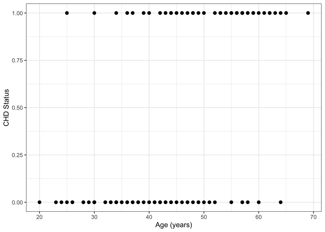
Figure 18.1: Plot of raw CHD data. Note that some points are overlapping here.
| Age Group | Proportion CHD |
|---|---|
| [17.5,22.5] | 0.000 |
| (22.5,27.5] | 0.167 |
| (27.5,32.5] | 0.091 |
| (32.5,37.5] | 0.200 |
| (37.5,42.5] | 0.250 |
| (42.5,47.5] | 0.429 |
| (47.5,52.5] | 0.455 |
| (52.5,57.5] | 0.800 |
| (57.5,62.5] | 0.800 |
| (62.5,67.5] | 0.750 |
| (67.5,72.5] | 1.000 |
How can we model this data?
- For an individual, we observe \(CHD = 1\) or \(CHD = 0\).
- Let \(p(x)\) denote the probability that \(CHD = 1\) for someone of age \(x\):
\[p(x) = P(CHD = 1 | Age = x)\]
What about \(p(x) = \beta_0 + \beta_1 x\)?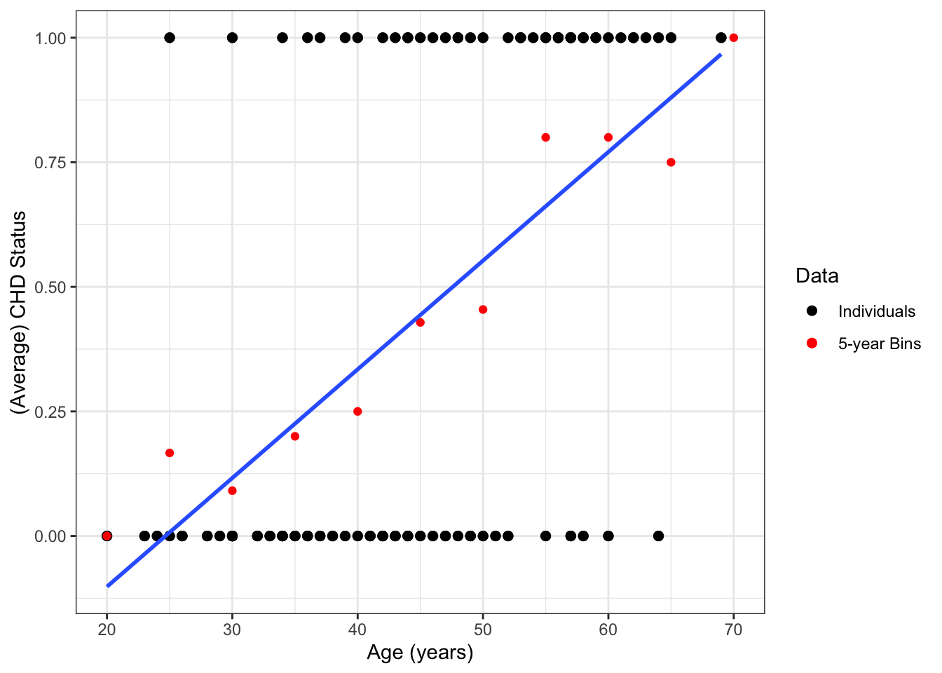
Figure 18.2: A simple linear regression line fit to the CHD data. Red dots show the average rates for five-year age bins.
The regression line in Figure 18.2 extends beyond the range of the data, giving nonsensical values below 25 years of age and above 70 years of age.
In settings like Example 18.1, it is no longer appropriate to fit a straight line through the data. Instead, we need a model that accommodate the limited range of outcome points (between 0 and 1) while still allowing for fitted values to differ by age (the predictor variable).
The key to doing this is the logistic function.
18.1 Logistic and Logit Functions
18.1.1 Logistic Function
The logistic function is given by the equation \[\begin{equation} f(\eta) = \frac{\exp(\eta)}{1 + \exp(\eta)} = \frac{1}{1 + \exp(-\eta)} \tag{18.1} \end{equation}\] and is plotted in Figure 18.3. Key features of the logistic function are:
- As \(\eta \to \infty\), \(f(\eta) \to 1\)
- As \(\eta \to -\infty\), \(f(\eta) \to 0\)
- \(f(0) = 1/2\)
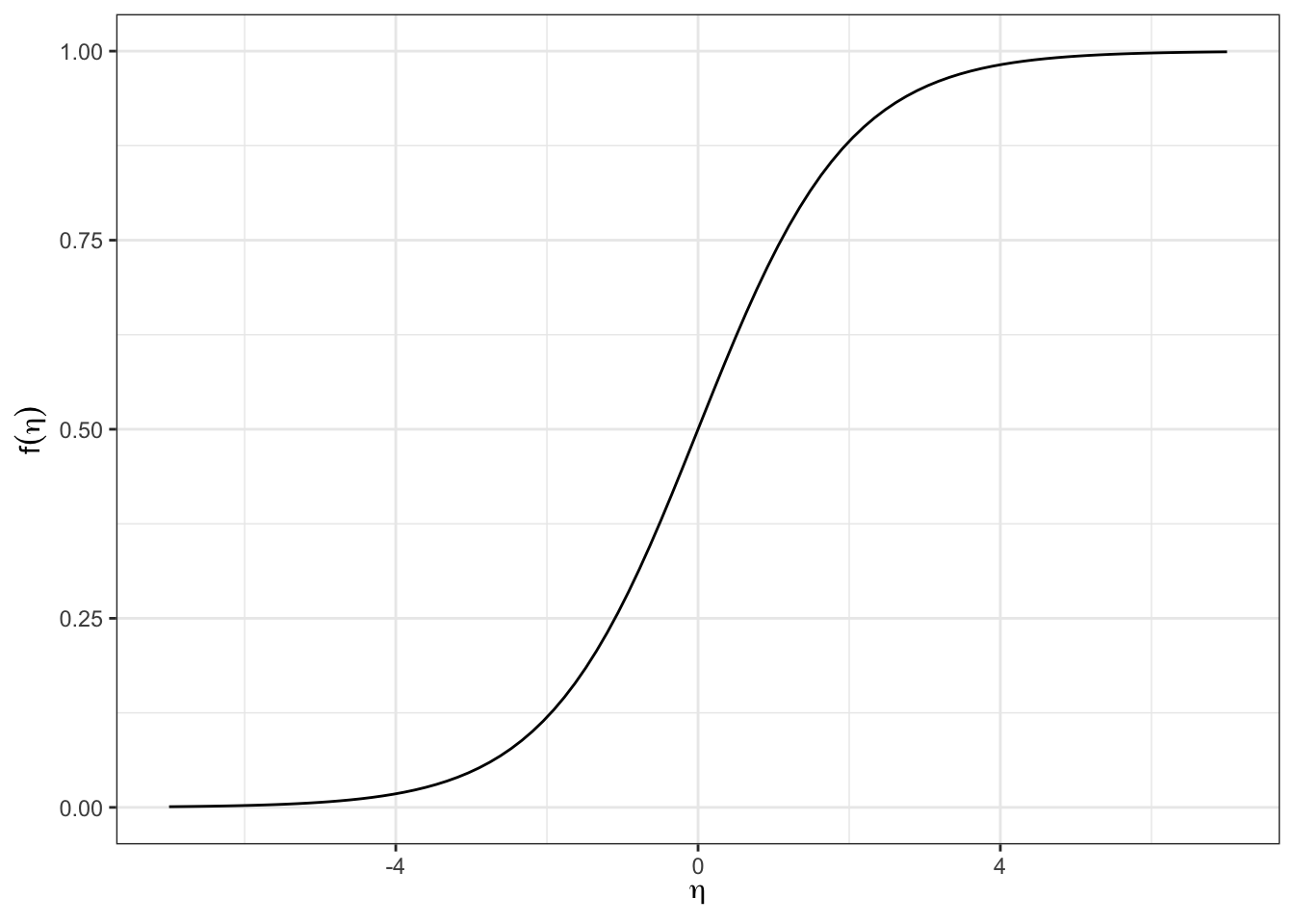
Figure 18.3: The logistic function.
While Figure 18.3 shows the logistic function in terms of \(\eta\), it is common to write \(\eta\) as a function of \(x\). Figure 18.4 shows this for several different relationships of the form \(\eta = \beta_0 + \beta_1x\). In that figure, we can see how the logistic function can be shifted and scaled depending upon the values of \(\beta_0\) and \(\beta_1\). This is analogous to modifying the equation for a line using its intercept and slope.
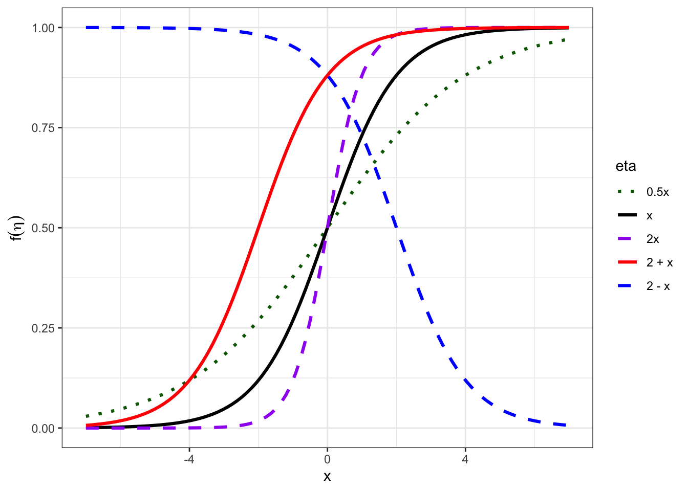
Figure 18.4: The logistic function for different settings of eta.
18.1.2 Logistic Regression
Logistic regression models the probability of an outcome using the logistic function:
\[\begin{equation} P(Y_i=1 | X_i=x) = p(x) = \frac{1}{1 + \exp\left(-\left[\beta_0 + \beta_1x\right]\right)} \tag{18.2} \end{equation}\]
Why use the logistic function?
- Inputs any value \((-\infty, \infty)\)
- Outputs a value between 0 and 1
- Provides smooth link between continuous predictor (\(\eta = \beta_0 +\beta_1x\)) and a probability \(P(Y=1)\).
Example 18.2 In the CHD data from Example 18.1, we can fit the equation: \(P(CHD =1 | Age = x) = \dfrac{1}{1 + \exp\left(-\left[-5.31 + 0.11x\right]\right)}\)

The logistic regression equation (18.2) implies a linear model for the log odds (= logit) of Y=1:
\[\begin{equation} logit(p(x)) = \log \frac{p(x)}{1-p(x)} = \beta_0 + \beta_1x \tag{18.3} \end{equation}\]
Mathematically, this connection can be derived by solving the logistic function (18.1) for \(\eta\): \[\begin{align*} p &= \frac{1}{1 + \exp(-\eta)}\\ p &= \frac{\exp(\eta)}{1 + \exp(\eta)}\\ p(1 + \exp(\eta)) &= \exp(\eta)\\ p + p\exp(\eta)) &= \exp(\eta)\\ p &= \exp(\eta) - p\exp(\eta)\\ p &= (1- p)\exp(\eta)\\ \frac{p}{1-p} &= \exp(\eta)\\ \log\left(\frac{p}{1-p}\right) &= \eta \end{align*}\]
Note similarity between (18.3) and the equation for simple linear regression: \(\E[Y] = \mu = \beta_0 + \beta_1x\). In both cases, there is a single “intercept” and “slope”, although those parameters have a different effect in the two models.
18.1.3 Odds
The odds of an event happening is the probability that it happens divided by the probability that it does not happen
\[Odds = \frac{p}{1 -p}\]
- Odds are always positive
- Higher odds means higher probability of success; lower odds means lower probability of success
- Odds are most commonly used in logistic regression and in sports betting
Example 18.3 If probability of winning a game is 0.67, the odds of winning are \(\dfrac{0.67}{1-0.67} = \dfrac{0.67}{0.33} = 2\)
18.2 Logistic Regression in R
18.2.1 Fitting Logistic Regression in R
In logistic regression, parameters (\(\beta\)’s) are estimated via maximum likelihood. The details of this procedure are covered in Section 19.
Obtaining estimates in R is similar to simple linear regression, except we use glm instead of lm:
chd_glm <- glm(chd~age, data=chdage, family=binomial)- First argument is a formula:
y ~ x1 + x2 + ... - The
dataargument is optional, but highly recommended.dataaccepts a data frame and the function looks for the variable names in the formula as columns of this data frame. - Setting
family=binomialindicates that we are fitting a logistic regression model (as opposed to other GLM). summary()andtidy()provide information similar to linear regression.
chd_glm##
## Call: glm(formula = chd ~ age, family = binomial, data = chdage)
##
## Coefficients:
## (Intercept) age
## -5.3095 0.1109
##
## Degrees of Freedom: 99 Total (i.e. Null); 98 Residual
## Null Deviance: 136.7
## Residual Deviance: 107.4 AIC: 111.4summary(chd_glm)##
## Call:
## glm(formula = chd ~ age, family = binomial, data = chdage)
##
## Deviance Residuals:
## Min 1Q Median 3Q Max
## -1.9718 -0.8456 -0.4576 0.8253 2.2859
##
## Coefficients:
## Estimate Std. Error z value Pr(>|z|)
## (Intercept) -5.30945 1.13365 -4.683 2.82e-06 ***
## age 0.11092 0.02406 4.610 4.02e-06 ***
## ---
## Signif. codes: 0 '***' 0.001 '**' 0.01 '*' 0.05 '.' 0.1 ' ' 1
##
## (Dispersion parameter for binomial family taken to be 1)
##
## Null deviance: 136.66 on 99 degrees of freedom
## Residual deviance: 107.35 on 98 degrees of freedom
## AIC: 111.35
##
## Number of Fisher Scoring iterations: 4tidy(chd_glm)## # A tibble: 2 × 5
## term estimate std.error statistic p.value
## <chr> <dbl> <dbl> <dbl> <dbl>
## 1 (Intercept) -5.31 1.13 -4.68 0.00000282
## 2 age 0.111 0.0241 4.61 0.0000040218.3 Risk Ratios and Odds Ratios
18.3.1 Calculating Quantities in Logistic Regression
The fitted logistic regression model is:
\[logit(\hat{p}(x)) = \log \frac{\hat{p}(x)}{1-\hat{p}(x)} = \hat\beta_0 + \hat{\beta}_1x\]
Or, equivalently:
\[ \hat{p}(x) = \frac{1}{1 + \exp\left(-\left[\hat{\beta}_0 + \hat{\beta}_1x\right]\right)}\]
Using this model, we can calculate the estimated
- The probability \(\hat{p}(x)\) of success. In some contexts (e.g., medicine), this is called the risk.
- risk ratio \(\dfrac{\hat{p}(x_1)}{\hat{p}(x_2)}\). This is the ratio of probabilities of success for two different values of the predictor variable.
- The **odds(()) \(\dfrac{\hat{p}(x)}{1 - \hat{p}(x)}\)
- The odds ratio \(\dfrac{\hat{p}(x_1)}{1 - \hat{p}(x_1)}\Bigg/\dfrac{\hat{p}(x_2)}{1 - \hat{p}(x_2)}\)
18.3.2 Calculating Risk of CHD
Example 18.4 Using the model from Example 18.2, what is the risk of CHD for a 65-year-old person? How does this compare to the risk of CHD for a 64-year-old person?
We estimate \(p(x)\) by plugging in our estimates of \(\beta_0\) and \(\beta_1\). \[\begin{align*} \hat{p}(65) & = \frac{1}{1 + \exp\left(-\left[\hat\beta_0 + \hat\beta_1 (65)\right]\right)} \\ & = \frac{1}{1 + \exp\left(-\left[-5.309 + 0.111 (65)\right]\right)} \\ &= 0.870 \end{align*}\] “We estimate that the probability of CHD for a 65 year-old person (from this population) is 0.870”
For 64-year-olds, the probablity of CHD is: \[\begin{align*} \hat{p}(64) & = \frac{1}{1 + \exp\left(-\left[-5.31 + 0.11 (64)\right]\right)} = 0.857 \end{align*}\] Thus, the risk ratio (RR) for CHD comparing 65- to 64-year-olds is: \[RR = \frac{0.870}{0.857} = 1.02\] “We estimate that the risk of CHD for a 65 year-old person is 2% greater than that for a 64 year-old person in this population.”
Example 18.5 We can calculate the risk and risk ratio of CHD for other ages:
| \(x\) | \(\hat{p}(x)\) | ||
|---|---|---|---|
| 65 | 0.870 | ||
| 64 | 0.857 | ||
| 51 | 0.586 | ||
| 50 | 0.559 | ||
| 31 | 0.133 | ||
| 30 | 0.121 |
| Age Comparison | Risk Ratio (RR) |
|---|---|
| 65 v 64 | 0.870/0.857 = 1.015 |
| 51 v 50 | 0.586/0.559 = 1.049 |
| 31 v 30 | 0.133/0.121 = 1.102 |
An important result from these tables is that the RRs are not constant! This is because the estimated probabilities are points along this (non-linear!) curve:
## `geom_smooth()` using formula = 'y ~ x'
18.3.3 Calculating the Odds
In addition to estimated risk (\(\hat{p}\)), we can calculate the odds that \(Y=1\): \[\begin{align*} \text{Odds of CHD for age $x$} &= odds(x) \\ & = \frac{p(x)}{1 - p(x)}\\ & = \exp\left(logit\left(p(x)\right)\right)\\ & = \exp\left(\beta_0 + \beta_1 x\right) \end{align*}\]
Example 18.6 What are the odds of CHD comparing 65 to 64-year-olds?
Plug in our parameter estimates: \[\begin{align*} \widehat{odds}(65) &= \exp\left(\hat\beta_0 + \hat\beta_1 (65)\right) \\ &= \exp(-5.309 + 0.111 * 65) \\ &= \exp(1.90) \\ &= 6.69 \end{align*}\] “We estimate that the odds of CHD for a 65 year-old person (from this population) to be 6.69” Note that \(\frac{0.870}{1 - 0.870} = 6.69\) and \(\frac{6.69}{1 + 6.69} = 0.870\). What about for 64 year-olds? \[\begin{align*} \widehat{Odds}(64) &= \exp(-5.309 + 0.111 * 64) \\ &= \exp(1.790) \\ &= 5.986 \end{align*}\] So we have:
| \(x\) | \(\widehat{log Odds}(x)\) | \(\widehat{Odds}(x)\) | \(\hat{p}(x)\) |
|---|---|---|---|
| 65 | 1.900 | 6.689 | 0.870 |
| 64 | 1.790 | 5.986 | 0.857 |
The odds ratio for CHD comparing 65- to 64-year-olds is: \[\frac{6.689}{5.986} = 1.117\]
We can do this for other ages:
| \(x\) | \(\widehat{log Odds}(x)\) | \(\widehat{Odds}(x)\) | \(\hat{p}(x)\) |
|---|---|---|---|
| 65 | 1.900 | 6.689 | 0.870 |
| 64 | 1.789 | 5.986 | 0.857 |
| 51 | 0.347 | 1.416 | 0.586 |
| 50 | 0.237 | 1.267 | 0.559 |
| 31 | -1.871 | 0.154 | 0.133 |
| 30 | -1.982 | 0.138 | 0.121 |
Odds ratios for CHD are:
| Age Comparison | Odds Ratio (OR) |
|---|---|
| 65 v 64 | 6.689/5.986 = 1.117 |
| 51 v 50 | 1.416/1.267 = 1.117 |
| 31 v 30 | 0.154/0.138 = 1.117 |
The ORs are constant!
The reason the ORs are constant are because the log-odds regression line is a straight line!

18.4 Interpreting \(\beta_1\) and \(\beta_0\)
18.4.1 Interpreting \(\beta_1\)
When comparing individuals who differ in age by 1 year,
- additive difference in log-odds is constant
- multiplicative difference in odds (i.e. odds ratio) is constant
- additive and multiplicative differences in risk depend on the specific ages
The logistic model is a linear model for the log-odds: \[\log\left(\frac{p(x)}{1 - p(x)}\right) = \beta_0 + \beta_1 x\]
Differences of one-unit in \(x\) correspond to a \(\beta_1\) difference in log-odds.
\[\begin{align*} log(odds(x+1)) - \,&\\ log(odds(x)) &= \log\left(\frac{p(x+1)}{1 - p(x+1)}\right) - \log\left(\frac{p(x)}{1 - p(x)}\right)\\ &= \left[\beta_0 + \beta_1 (x + 1)\right] - \left[\beta_0 + \beta_1 x\right] \\ & = \beta_0 + \beta_1x + \beta_1 - \beta_0 -\beta_1x\\ & = \beta_1 \end{align*}\]
Additive differences in log-odds are multiplicative differences in odds:
\[\begin{align*} log(odds(x+1)) - log(odds(x)) &= \beta_1 \\ \exp\left[log(odds(x+1)) - log(odds(x))\right] &= \exp(\beta_1) \\ \frac{\exp[log(odds(x+1))]}{\exp[log(odds(x))]} &= \exp(\beta_1) \\ \frac{odds(x+1)}{odds(x)} &= \exp(\beta_1) \\ \end{align*}\]
18.4.2 Interpreting \(\beta_1\): CHD Example
Odds ratios for CHD are:
| Age Comparison | Odds Ratio (OR) |
|---|---|
| 65 v 64 | 6.689/5.986 = 1.117 |
| 51 v 50 | 1.416/1.267 = 1.117 |
| 31 v 30 | 0.154/0.138 = 1.117 |
\[\hat\beta_1 = 0.11 \Rightarrow \exp(0.11) = 1.117\]
In this population, a difference of one-year in age is associated, on average, with 11.7% higher odds of CHD.
18.4.3 Interpreting \(\beta_0\)
The logistic model is a linear model for the log-odds: \[\log\left(\frac{p(x)}{1 - p(x)}\right) = \beta_0 + \beta_1 x\]
What is \(\beta_0\)?
\[\beta_0 = \log\left(\frac{p(0)}{1 - p(0)}\right)\]
- The “intercept” for the log-odds
- The log-odds when \(x=0\).
- In most cases, this is of little scientific interest
- In some cases, this has no scientific meaning
18.4.4 Calculating Odds Ratios and Probabilities in R
- As with linear regression, avoiding rounding in intermediate steps when computing quantities
- Instead, use R functions that carry forward full precision
The tedious approach:
coef(chd_glm)## (Intercept) age
## -5.3094534 0.11092111/(1 + exp(-(coef(chd_glm)[1] + coef(chd_glm)[2]*64)))## (Intercept)
## 0.8568659The recommended approach: use predict()
- Set
type="link"to compute estimated log-odds - Set
type="response"to compute estimated probabilities
predict(chd_glm, newdata=data.frame(age=64),
        type="link")
## 1
## 1.7895predict(chd_glm, newdata=data.frame(age=64),
type="response")## 1
## 0.8568659Example 18.7 Data are available on the first round of the 2013 Women’s U.S. Tennis Open. Let’s model the probability of the player winning (variable won) as a function of the number of unforced errors and double faults she made (variable fault_err).

open_mod1 <- glm(won~fault_err,
                 data=usopen,
family=binomial)summary(open_mod1)##
## Call:
## glm(formula = won ~ fault_err, family = binomial, data = usopen)
##
## Deviance Residuals:
## Min 1Q Median 3Q Max
## -1.7707 -1.0743 0.4906 0.9316 1.4243
##
## Coefficients:
## Estimate Std. Error z value Pr(>|z|)
## (Intercept) 3.23139 1.50329 2.150 0.0316 *
## fault_err -0.09036 0.04322 -2.091 0.0366 *
## ---
## Signif. codes: 0 '***' 0.001 '**' 0.01 '*' 0.05 '.' 0.1 ' ' 1
##
## (Dispersion parameter for binomial family taken to be 1)
##
## Null deviance: 37.096 on 26 degrees of freedom
## Residual deviance: 30.640 on 25 degrees of freedom
## AIC: 34.64
##
## Number of Fisher Scoring iterations: 4tidy(open_mod1, conf.int=TRUE)## # A tibble: 2 × 7
## term estimate std.error statistic p.value conf.low conf.high
## <chr> <dbl> <dbl> <dbl> <dbl> <dbl> <dbl>
## 1 (Intercept) 3.23 1.50 2.15 0.0316 0.694 6.80
## 2 fault_err -0.0904 0.0432 -2.09 0.0366 -0.193 -0.0182tidy(open_mod1, conf.int=TRUE, exp=T)## # A tibble: 2 × 7
## term estimate std.error statistic p.value conf.low conf.high
## <chr> <dbl> <dbl> <dbl> <dbl> <dbl> <dbl>
## 1 (Intercept) 25.3 1.50 2.15 0.0316 2.00 897.
## 2 fault_err 0.914 0.0432 -2.09 0.0366 0.824 0.982In this model, we can interpret \(\hat\beta_1 = -0.09\) and \(\exp(\hat\beta_1) = \exp(-0.09) = 0.914\) as
- A difference of 1 fault or error is associated with an estimated difference of 0.09 lower log odds (95% CI: -0.193, -0.018) of winning a tennis match at the 2013 US Open.
- A difference of 1 fault or error is associated with an estimated odds ratio of 0.914 (95% CI: 0.824, 0.982) for winning a tennis match at the 2013 US Open.
18.5 Multiple Logistic Regression
In our examples so far, we have considered only one predictor variable. Almost all practical analyses consider multiple predictor variables. This leads to multiple logistic regression.
18.5.1 Coefficient Interpretation
\[logit(p_i) = \beta_0 + \beta_1x_{i1} + \beta_2x_{i2} + \dots + \beta_kx_{ik}\] \(\exp(c\beta_k)\) is the odds ratio for a \(c\)-unit difference in variable \(k\), when all other variables are held constant.
- In practice, the log odds do not lie on a perfectly straight line.
- We are estimating a general trend in the data
“On average, the odds of [outcome] are \(\exp(c\beta_k)\) times larger for every c-unit difference in [variable \(k\)] among observations with the same values of the other variables.”