Chapter 7 Other Topics in SLR
This chapter covers several different variations of the simple linear regression model. The fundamental aspects of the model do not change, but the interpretations of parameters are impacted by transformations to the predictor and outcome variables.
7.1 Regression with Centered \(x\)
One common variation of the SLR model is to center the predictor variable, which means we use \(x_i - \overline{x}\) instead of \(x_i\).
We can re-arrange the SLR model equation as: \[\begin{align*} Y_i &= \beta_0 + \beta_1x_i + \epsilon_i \\ &= \beta_0 + \beta_1x_i - \beta_1\overline{x} + \beta_1\overline{x} + \epsilon_i \\ &= {\color{blue}{\beta_0 + \beta_1\overline{x}}} + \beta_1 (x_i - \overline{x}) + \epsilon_i \\ &= {\color{blue}{\beta_0'}} + \beta_1 (x_i - \overline{x}) + \epsilon_i \end{align*}\]
Thus, we still have an SLR model, but with \(\beta_0'\) in place of \(\beta_0\). From the derivation above, we can see that \(\beta_0' = \beta_0 + \beta_1\overline{x}\). In words, this means that \(\beta_0'\) is the mean of \(Y\) for observations with the average value of the predictor variable. This is the primary reason for centering the \(x\) variable, since it has a practical meaning, often unlike the intercept from an uncentered model.
The slope parameter \(\beta_1\) is unchanged by this reparameterization. The model inference–hypothesis tests and confidence intervals–are not changed by centering the \(x\) variable.
Graphically, centering the predictor variable is equivalent to using the point (\(\overline{x}, \overline{y}\)) as the origin (see Figure 7.1). This has no impact on the slope of the regression line, but does affect the intercept.
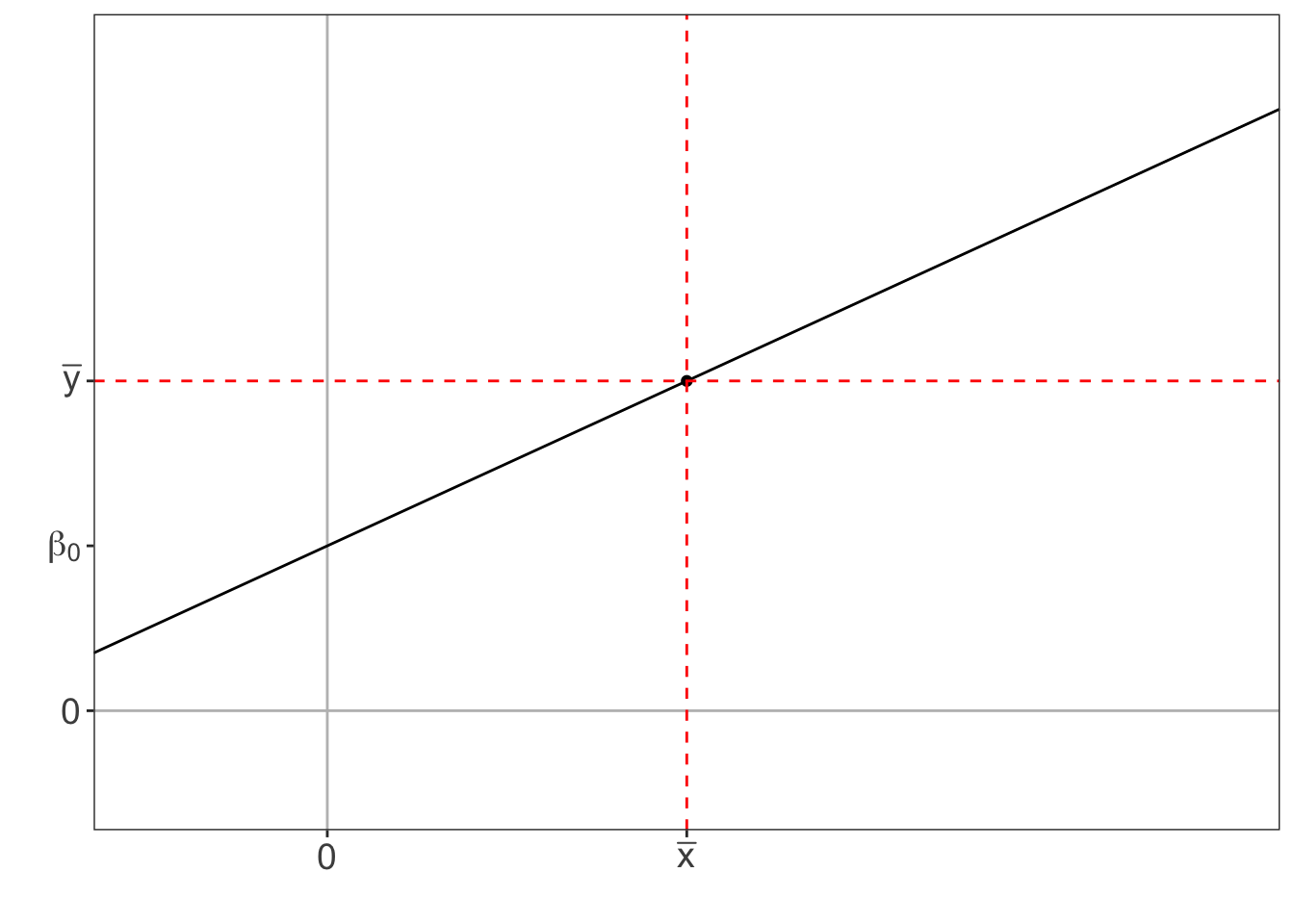
Figure 7.1: Shifting the origin to the average of the data.
First, we need to create the centered variable:
penguins <- penguins %>%
   mutate(flipper_length_mm_centered=flipper_length_mm - mean(flipper_length_mm, na.rm=TRUE))
When we fit the SLR model with this centered variable, we get point estimates \(\hat\beta_0 = 4201.8\) and \(\hat\beta_1 = 49.7\). As expected, the slope is the same as the uncentered model. The estimated average body mass for penguins with “average” flipper length is 4,202 grams. Since the SLR line passes through (\(\overline{x}, \overline{y})\), this is exactly the mean penguin body mass in this data.
7.2 Rescaling Units
7.2.1 Rescaling \(x\)
In addition to centering, another common transformation is to scale a variable. When the predictor variable is scaled by a factor \(c\), the value of \(\beta_1\) (and thus \(\hat\beta_1\)) is scaled by \(1/c\). This can be verified mathematically by re-arranging the SLR equation: \[\begin{align*} Y_i &= \beta_0 + \beta_1 x_i + \epsilon_i \\ &= \beta_0 + \frac{\beta_1}{c} (cx_i) + \epsilon_i\\ &= \beta_0 + \tilde{\beta_1} \tilde{x_i} + \epsilon_i \end{align*}\] where \(\tilde{x}_i = cx_i\) and \(\tilde{\beta}_1 = \beta_1/c\).
In principle, predictor variables can be rescaled by any value, but the most common is scaling by its standard deviation. Together with centering the variable, this is known as standardization of the predictor variable. This leads to \(\beta_1\) representing the difference in the average value of the outcome for a one-standard deviation difference in \(x\). Other common scaling factors are: factors of 10 or other values that can change units (e.g., going from kilometers to meters) and the interquartile range (IQR) of \(x\).
scale() command:
penguins <- penguins %>%
   mutate(flipper_length_mm_standardized=scale(flipper_length_mm))
If we fit a SLR model with this standardized version of flipper length, we obtain \(\hat\beta_0 = 4201.8\) and \(\hat\beta_1 = 698.7\). The scaling of \(x\) had not impact on the point estimate \(\hat\beta_0\), but did change the value of \(\hat\beta_1\). From this model, an interpreation statement for \(\hat\beta_1\) is: A one standard deviation difference in flipper length is associated with a difference of 699 grams in average body mass (95% CI: 657, 741).
This demonstrates one advantage to scaling by the standard deviation: it can simplify interpretations of the slope parameter, particularly in contexts where the audience may not be familiar with the practical importance of a 1-unit difference in the predictor. For example, someone who is not familiar with the average lengths of penguin flippers may not have a good sense of how large a 1 mm difference in flipper length is. Does it represent a small, but important, amount? Or is it a negligible difference? The same reader could understand that a one-standard deviation difference in flipper length is a meaningfully large difference in flipper length. However, when reporting results from a model with a standardized predictor, it is still important to report what the magnitude of the standard deviation is.
Rescaling the predictor variable has no impact on the inferential conclusions about the model. Any multiplicative change in \(\hat\beta_1\) due to scaling also impacts \(se(\hat\beta_1)\) by the same factor, and so the test statistics for hypothesis tests remain unchanged.
7.2.2 Rescaling \(Y\)
It is also possible to rescale the outcome variable. This is generally only done when changing units; it is uncommon to standardize the outcome variable. The impact on the regression parameters can again be computed by rearranging the SLR model equation: \[\begin{align*} Y_i &= \beta_0 + \beta_1x_i + \epsilon_i \\ cY_i &= c\beta_0 + c\beta_1x_i + c\epsilon_i \\ \tilde{Y}_i &= \tilde{\beta}_0 + \tilde{\beta}_1x_i + \tilde{\epsilon_i} \end{align*}\] where \(\tilde{Y}_i = cY_i\), \(\tilde\beta_0 = c\beta_0\), \(\tilde{\beta}_1 = c\beta_1\) and \({\rm Var}(\tilde{\epsilon}_i) = c^2\sigma^2\).
Unlike rescaling \(x\), which only impacted \(\beta_1\), rescaling the outcome variable affects all three parameters in the SLR model. However, once again the inferential conclusions are not changed since the numerator and denominator in the test statistic are multiplied by the same factor.